Vector potential, far field and the Fraunhofer distance
The retarded vector potential, the far-field approximation, transverse fields, the Fraunhofer distance proved, reactive, Fresnel and Fraunhofer regions, the short dipole in three lines.
To compute the field of an arbitrary antenna one does not solve Maxwell’s equations from scratch every time. One goes through the vector potential, obtained from the currents with an integral, and far from the antenna the formulas simplify a great deal. In this lesson we look at the retarded vector potential, the far-field approximation and the resulting field, the proof of the Fraunhofer distance, the three regions around an antenna and the example of the short dipole.
The vector potential
With sinusoidal currents of angular frequency  , the magnetic field is written as the curl of a vector potential,
 , and with the Lorenz gauge the potential satisfies the Helmholtz equation with a source,
 , with
 (lesson on plane waves). The solution is the retarded potential:

Every current element contributes a spherical wave starting from its position: the factor  is the propagation delay,
 the spherical attenuation. Once
 is known, the fields follow by differentiation.
The far-field approximation
Put the origin inside the antenna, of maximum dimension  , and observe at distance
 in a direction forming the angle
 with the vector
 of a source point.
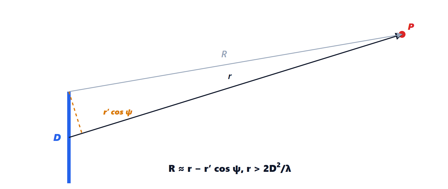
Expanding the distance:  . In the denominator ,
 is enough; in the exponent, instead, distance differences matter even if small, because they are compared with the wavelength. Keep
 and neglect the quadratic term. Then

The integral depends only on the direction  : it is a kind of spatial Fourier transform of the current distribution. The far field is a spherical wave, varying as
 , modulated by a function of direction alone. The fields are transverse:

with  : locally a plane wave.
The Fraunhofer distance
Theorem. The phase error due to the neglected term is at most  if

Proof. The term neglected in the exponent is  . It is largest for points at the edge of the antenna,
 , and for
 : it equals
 . Requiring it not to exceed :
 , i.e.
 . ∎
A phase error of (22.5°) barely alters the main lobe and the gain, and it is the convention used in all measurements. Example. A 1 m dish at 10 GHz ( cm) has its Fraunhofer distance at
 m: measuring its pattern requires long ranges or the techniques of the lesson on measurements.
The three regions
Around an antenna one distinguishes:
- the reactive near field, within about
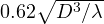 (for small antennas, about
 ): energy is mainly stored and exchanged with the antenna, as in the field of a capacitor or an inductor;
- the radiating near field (Fresnel region), up to
 : energy propagates, but the shape of the pattern still depends on distance;
- the far field (Fraunhofer region), beyond : the pattern no longer changes with distance, and the field falls off as
 .
13.56 MHz RFID antennas and wireless charging work in the reactive near field, with inductive coupling; radio communications in the far field.
The example of the short dipole
A wire of length  along the
 axis, carrying a uniform current
 , has potential
 . Its component along
 is
 , and therefore
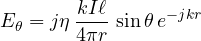
the same result obtained in the Electromagnetic Fields lesson on the elementary dipole, but in three lines. The pattern is  in power: zero along the wire, maximum in the perpendicular plane. With the same procedure, integrating over different currents, the long dipoles, arrays and apertures of the next lessons are computed.