Stability: eigenvalues, BIBO stability and the Lyapunov equation
Lyapunov's definitions of stability, the eigenvalue criterion proved, marginal stability, input-output stability and hidden modes, the Lyapunov equation with proof of the theorem.
Stability is the first property required of a system: a small disturbance must not drive it far away. But “stable” has different meanings, and the difference matters: a system can give bounded outputs for every bounded input and hide inside it a mode that blows up. In this lesson we look at Lyapunov’s definitions, the eigenvalue criterion with proof, input-output stability and its difference from internal stability, and the Lyapunov equation with the proof of the theorem.
Definitions
We consider the free response around an equilibrium, which for a linear system can be moved to the origin.
- The equilibrium is stable (in the sense of Lyapunov) if for every
 there exists
 such that, starting at a distance less than
 , the state stays forever at a distance less than
 . In words: starting close enough, one stays close.
- It is asymptotically stable if it is stable and moreover the state tends to the equilibrium.
- It is unstable if it is not stable.
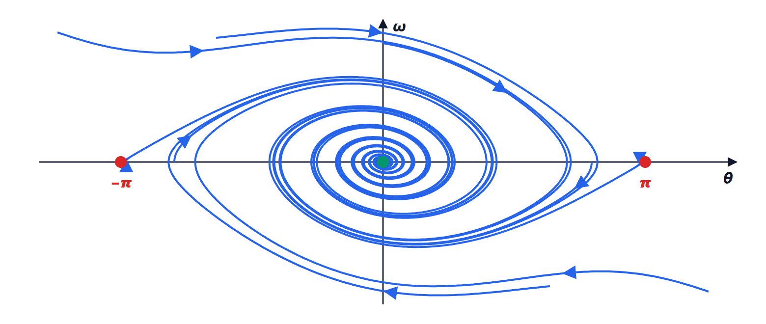
A frictionless pendulum hanging down is stable but not asymptotically: it oscillates forever with its initial amplitude. With friction it becomes asymptotically stable. The inverted pendulum is unstable.
The eigenvalue criterion
For linear time-invariant systems stability is a property of the system, not of a single equilibrium, and it is read from the eigenvalues of  .
Theorem. The system  is asymptotically stable if and only if all the eigenvalues of have strictly negative real part.
Proof. The free response is 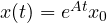 , and every element of
 is a combination of the modes
 (lesson on the solution), with
 less than the multiplicity of the eigenvalue. If all
 , every mode tends to zero, because the decaying exponential beats any power of
 : so
 , and
 from every initial state. Moreover
 is bounded, which gives stability. Conversely, if an eigenvalue has
 , starting from its eigenvector (or its real part, if complex) the evolution
 does not tend to zero. ∎
The borderline case: if the eigenvalues with zero real part have Jordan blocks of size 1 (i.e. enough eigenvectors), the system is marginally stable, like the frictionless oscillator. If not, growing modes  appear, as in the double integrator
 , which with a non-zero initial velocity drifts away forever. In discrete time the criterion is the same with
 . To check it without computing the eigenvalues, the Routh-Hurwitz criterion is applied to the characteristic polynomial (Automatic Control lesson on stability).
Internal stability and input-output stability
A system is BIBO stable (bounded input, bounded output) if every bounded input gives a bounded output, starting from zero state. It is checked on the transfer function: all the poles of  must have negative real part.
Asymptotic stability implies BIBO stability, because the poles of are among the eigenvalues of . The converse does not hold: if an unstable eigenvalue cancels with a zero in the transfer function, the corresponding mode does not appear in the output, but it is there.
Example. With 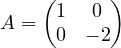 ,
 ,
 one gets
 : BIBO stable. But the first state evolves as
 , and any noise or initial condition makes it grow without bound, until something saturates or breaks. The unstable mode is not reachable from the input, which is why the transfer function does not see it (lessons on reachability and observability). The practical rule: never cancel an unstable pole with a zero of the controller.
The Lyapunov equation
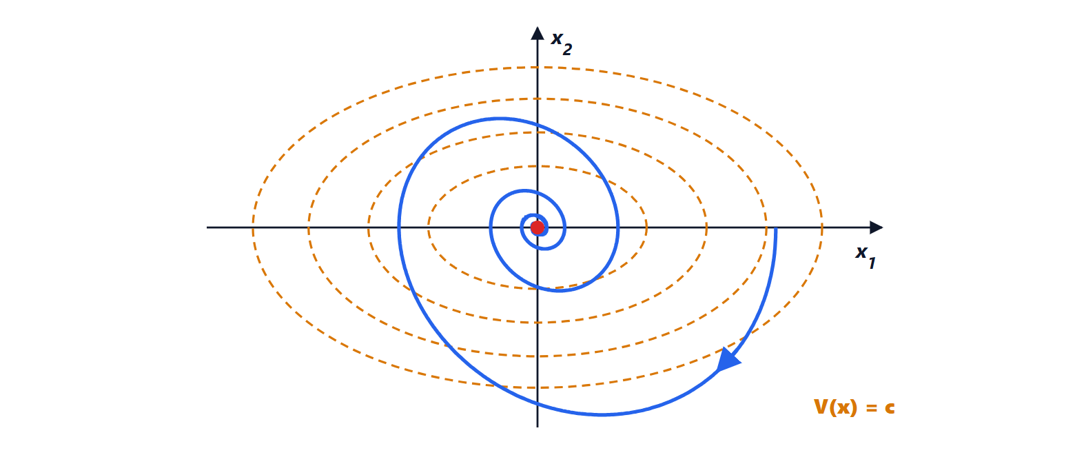
Lyapunov’s second method proves stability by finding an “energy” function that decreases along trajectories, without solving the equations. For linear systems a quadratic function  is sought, with
 symmetric and positive definite, so that
 for every
 and its level curves are ellipsoids around the origin.
Theorem. If there exist symmetric positive definite matrices and  such that

then the system is asymptotically stable.
Proof. Along a trajectory, the derivative of  is

which is negative for every . So  strictly decreases along every trajectory not at the origin. Since and are positive definite, there is
 with
 (one can take the ratio of the smallest eigenvalue of to the largest of ), so
 and
 : tends to zero exponentially, and so does
 . ∎
The converse also holds: if the system is asymptotically stable, for every positive definite the Lyapunov equation has a unique positive definite solution , given by  . In practice one chooses
 , solves the linear equation for and checks whether is positive definite. In discrete time the equation becomes
 .
The value of the method lies above all in non-linear systems, where eigenvalues are not enough (lesson on non-linear systems), and in the fact that also gives an estimate of how fast the state converges.