Discrete-time systems and exact discretisation
Solution of difference equations by induction, discrete modes and the unit circle, deadbeat response, exact discretisation proved, continuous and discrete eigenvalues, the z-transform.
Many systems evolve in steps: a computer updating its state at every cycle, a digital controller, a yearly economic model, a population that breeds by seasons. Discrete-time systems have the same theory as continuous ones, with matrix powers in place of exponentials and the unit circle in place of the left half-plane. In this lesson we look at the solution of difference equations with proof, discrete modes, the exact discretisation of a continuous system with its proof and the link between eigenvalues in the two worlds.
Discrete-time state equations
The discrete-time linear time-invariant system is

where  is an integer, the step index.
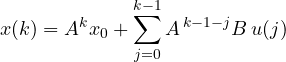
Theorem. The solution with  is
Proof. By induction. For  the sum is empty and
 remains. If the formula holds for , then

and the last term is exactly the term  of the sum, with
 . The formula therefore holds for
 . ∎
It is the discrete analogue of Lagrange’s formula: free response  plus a discrete convolution of the input with the impulse response
 .
Discrete-time modes
If  is diagonalisable,
 , and the modes are the sequences
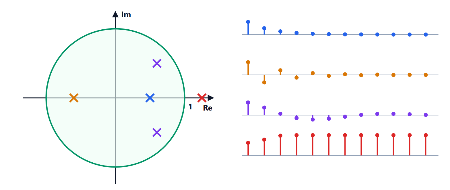
 . Their behaviour depends on the position of the eigenvalue in the complex plane relative to the circle of radius 1:
 : the mode tends to zero;
 : it diverges;
 real positive: monotonic behaviour; real negative: the sign alternates at every step, a behaviour with no equivalent in first-order continuous systems;
 complex: oscillation
 , with
 radians per step;
 : the mode vanishes after one step. If all the eigenvalues are zero,
 and any initial state is cleared in at most
 steps. This is the deadbeat response, impossible in continuous time.
Exact discretisation
A continuous system driven by a computer receives a piecewise-constant input: the computer updates it every  seconds and holds it until the next update (Process Control lesson on digital control). Seen only at the sampling instants, the continuous system becomes exactly a discrete system.
Theorem. If  and
 is constant for
 , then
 satisfies

Proof. Apply Lagrange’s formula starting at instant  for a duration :

With the change of variable  the integral becomes
 , and
 comes out of the integral because it is constant. ∎
It is not an approximation: at the sampling instants the two models coincide exactly.
Example. The first-order system  has
 ,
 . Then
 and
 . The static gain
 is the same as that of the continuous system, as it must be.
Eigenvalues in the two worlds
Theorem. If is an eigenvalue of  , then
 is an eigenvalue of
 , with the same eigenvector.
Proof. If  , then
 for every , and summing the exponential series
 . ∎
Since  , an eigenvalue in the left half-plane (
 ) goes inside the unit circle, the imaginary axis goes onto the circle, the right half-plane outside. Stability is preserved by sampling. Moreover, continuous eigenvalues differing by
 end up at the same point: this is aliasing (lesson on sampling) seen from the side of the modes.
The z-transform
Like the Laplace transform for continuous systems, the z-transform turns difference equations into algebraic ones:  becomes
 . The discrete transfer function is

and its poles are the eigenvalues of (unless there are cancellations). Stability requires them all to lie inside the unit circle.





