Matrix exponential, Lagrange's formula and natural modes
Definition and properties of the matrix exponential, Lagrange's formula proved, free and forced response, modes for real, complex and repeated eigenvalues, computation with Laplace, a complete example.
A linear time-invariant system  can be solved exactly, for any input. The solution is written with the matrix exponential, and its structure reveals the natural modes of the system: the elementary forms of motion of which every evolution is a combination. In this lesson we define the matrix exponential, prove Lagrange’s formula, look at the modes for real, complex and repeated eigenvalues, the computation with the Laplace transform and a complete example.
The matrix exponential
For a scalar,  has solution
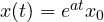 . For matrices it is defined in the same way, with the series

which converges for every square matrix and every  . Differentiating term by term gives
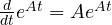 , and moreover
 and
 . Beware:
 holds only if
 and
 commute.
Lagrange’s formula
Theorem. The solution of with  is

Proof. Multiply the equation on the left by  :
 . The left-hand side is the derivative of
 , because
 ( commutes with its own exponential). Integrating from 0 to :

and multiplying on the left by  gives the formula. The solution is unique because the equation is linear with constant coefficients. ∎
The first term is the free response, due to the initial condition alone; the second the forced response, due to the input alone, and it is a convolution integral with the state impulse response  . The output is obtained by multiplying by
 and adding
 . It is the same structure as the convolution seen in the Signal Theory lesson on LTI systems.
Natural modes
If is diagonalisable,  with
 the diagonal matrix of eigenvalues and
 the matrix of eigenvectors. Then
 and, summing the series,

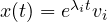
Every element of is therefore a combination of the functions  : the modes of the system. If the initial state is an eigenvector
 , the free response always stays along that direction,
 .
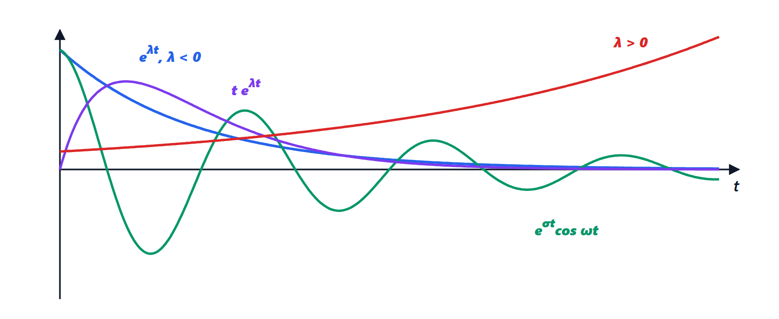
The possible cases are:
- real eigenvalue
 : mode
 , which decays if
 and diverges if
 ;
- complex pair
 : two complex conjugate modes which, combined, give the real functions
 and
 : an oscillation of angular frequency
 , damped or amplified according to the sign of
 ;
- repeated eigenvalue with fewer independent eigenvectors than its multiplicity: is not diagonalisable, the Jordan form is used, and the modes
 ,
 , and so on appear. For they decay anyway, because the exponential beats the power; for
 they give ramps, as in the double integrator.
Computation with the Laplace transform
Transforming gives  , i.e.
 . Comparing with Lagrange’s formula:

where  is the transfer function. Since
 , the poles of are among the eigenvalues of : they are all of them, unless there are cancellations (lesson on observability).
A complete example
Let 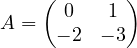 . The characteristic polynomial is
 , with eigenvalues
 and
 . One computes

and splits each element into partial fractions: for instance  . Inverting:

One checks at once that  gives the identity. Every element contains only the modes
 and
 : any initial condition dies out with two decaying exponentials, the slower of which has time constant 1. The dominant mode is the one with the least negative real part, which survives longest and sets the settling time.