Demand forecasting: moving averages and exponential smoothing
Moving average, exponential smoothing with weights and average age of data proved, a numerical example, MAD, MAPE and tracking signal, Holt and Holt-Winters methods.
Every logistics decision rests on a demand forecast: how much stock to hold, how many trucks to book, how much to produce next month. Forecasts are always wrong; the aim is for them to be only a little wrong, without systematic errors, and to know by how much. In this lesson we look at the moving average and exponential smoothing with the proof of its weights and of the average age of the data, a numerical example, error measures, and methods for trend and seasonality.
The moving average
The simplest forecast for the next period is the average of the last  values:
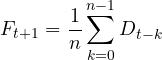
With large the forecast is stable but reacts slowly to changes; with small it reacts quickly but also chases noise. The average age of the data used is  periods.
Exponential smoothing
Exponential smoothing corrects the previous forecast by a fraction  of the error:

It requires storing a single number, and it is the most widely used method in inventory management systems. It is a first-order low-pass filter (lesson on discrete-time systems), like the burst estimate in CPU scheduling (Operating Systems lesson on scheduling).
Theorem. Expanding the recursion, the forecast is a weighted average of all past data with weights  , which sum to 1; the average age of the data is
 .
Proof. Repeatedly substituting  gives
 (the remainder, multiplied by
 , tends to zero). The sum of the weights is the geometric series
 . The average age is
 , using
 . ∎
The weights decrease geometrically: recent data count more, but none is entirely forgotten. Equating the average ages, smoothing with is equivalent to a moving average of  periods: with
 the average age is 4 periods, like a moving average of 9.
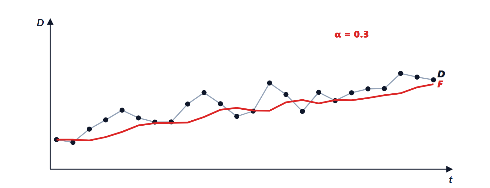
Example. Demand 100, 110, 105, 120, 115 in the first five months,  , initial forecast 100. The forecasts for months 2-6 are 100, 103, 103.6, 108.5, 110.5. The errors for months 2-5 are +10, +2, +16.4, +6.5: mean absolute deviation (MAD) about 8.7, but all positive.
Measuring error
- MAD (mean absolute deviation) or RMSE (root mean square error): how wrong one is on average; with roughly normal errors
 , which enters the safety stock calculation (lesson on inventory).
- MAPE (mean absolute percentage error): comparable across items with different volumes, but unusable with demands close to zero.
- Bias: the mean of the signed errors. It must be close to zero; the tracking signal, the cumulative sum of errors divided by the MAD, signals when it exceeds about ±4 that the model no longer follows demand.
In the example all errors are positive: simple smoothing chases a trend without catching it, because it assumes a constant level.
Trend and seasonality
- Holt’s method adds a second equation estimating the trend slope, also smoothed, and the forecast becomes level plus slope times the number of periods.
- The Holt-Winters method adds seasonal coefficients (for example demand for air conditioners in summer or electronics at Christmas), updated every year.
- Causal methods relate demand to explanatory variables (price, promotions, weather) by regression; machine learning methods combine many variables and many similar items.
Two practical rules apply to all: aggregate forecasts (by product family, region, month) are more accurate than detailed ones, by the same statistical compensation as the square-root law (lesson on the supply chain); and the further ahead one looks, the larger the error, so it pays to shorten response times rather than forecast further ahead.





