Inventory management: economic order quantity and reorder point
The economic order quantity proved with an example, cost robustness proved, safety stock and reorder point with an example, reorder-point and periodic-review systems.
Ordering small quantities often costs in orders and transport; ordering large quantities rarely costs in storage. The economic order quantity finds the compromise, and the reorder point establishes when to order so as not to run out. In this lesson we look at the economic order quantity formula with its proof, its surprising robustness proved, safety stock and the reorder point with a complete example, and the classification of reorder systems.
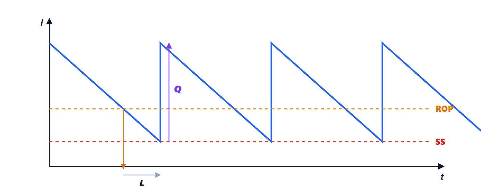
The economic order quantity
Consider an item with constant demand  units per year, a fixed cost
 per order (issuing, transport, receiving, inspection) and a holding cost
 per unit per year. Ordering batches of
 units, stock falls steadily from to zero, and averages
 .
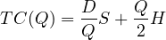
The total annual cost (excluding the purchase price, which does not depend on ) is
Theorem. The cost is minimum for the economic order quantity

and at that point ordering cost and holding cost are equal, with  .
Proof.  , which vanishes for
 ; the second derivative
 is positive, so it is a minimum. At that point
 , since this is equivalent to
 , and the sum of the two equal terms is
 . ∎
Example.  units per year,
 euros per order,
 euros per unit per year (20 % of a value of 10 euros):
 units, about 15 orders a year, cost
 euros.
Robustness
Theorem. Ordering a batch different from the optimum, the relative cost is
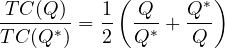
Proof. Dividing  by
 :
 , and
 . Adding gives the formula. ∎
The function  is very flat near 1: with a batch 29 % larger than the optimum (1000 units instead of 775) the cost rises by only 3.3 %, to 1600 euros. Batches can therefore be rounded to convenient quantities (a pallet, a case) with almost no loss, and errors in estimating and , which enter under a square root, matter little.
Safety stock and reorder point
Demand is not constant, and the order takes a time  to arrive. One reorders when stock falls to the reorder point

where  and
 are the mean and standard deviation of daily demand (assumed independent from day to day, so with variance over days equal to
 ), and
 sets the service level: with normal demand,
 gives a 95 % probability of not running out during the lead time. The second term is the safety stock.
Example. With 250 working days,  units a day;
 days;
 . Safety stock
 units;
 . Going from 95 % to 99 % (
 ) raises the safety stock to 78 units: the last percentage points of service cost more and more.
Reorder systems
- Reorder point (fixed quantity , variable interval): order when stock falls to
 ; it requires knowing the stock at every moment, which is easy with information systems.
- Periodic review (fixed interval
 , variable quantity): every days order what is needed to return to a target level; simpler to organise, but needs more safety stock, because it must cover
 days.
- For items whose demand depends on a production plan (components of a product), MRP is used instead (Business Management lesson on production planning).
The ABC classification (lesson on warehousing) shows where to invest attention: tight control and frequent reviews for the few high-value items, simple rules for the many low-value ones.





