Transistor amplifiers: operating point and small-signal model
Load line and operating point, transconductance of MOSFET and BJT, the small-signal model, the common-source amplifier, other configurations and the Miller effect.
A transistor amplifies because a small change in input voltage produces a large change in output current, which across a resistor becomes a large voltage change. To exploit it you must separate two problems: biasing, the DC voltages and currents that set the operating point, and the signal, the small changes around that point. In this lesson we look at the small-signal models of the MOSFET and the BJT and at the basic configurations.
Load line and operating point
Consider a MOSFET with its source grounded and its drain connected to the supply  through a resistor
 . By Kirchhoff’s law at the output,

This is a straight line in the  plane, the load line, running from on the voltage axis to
 on the current axis. The transistor must lie both on this line and on its characteristic: the intersection is the operating point Q.
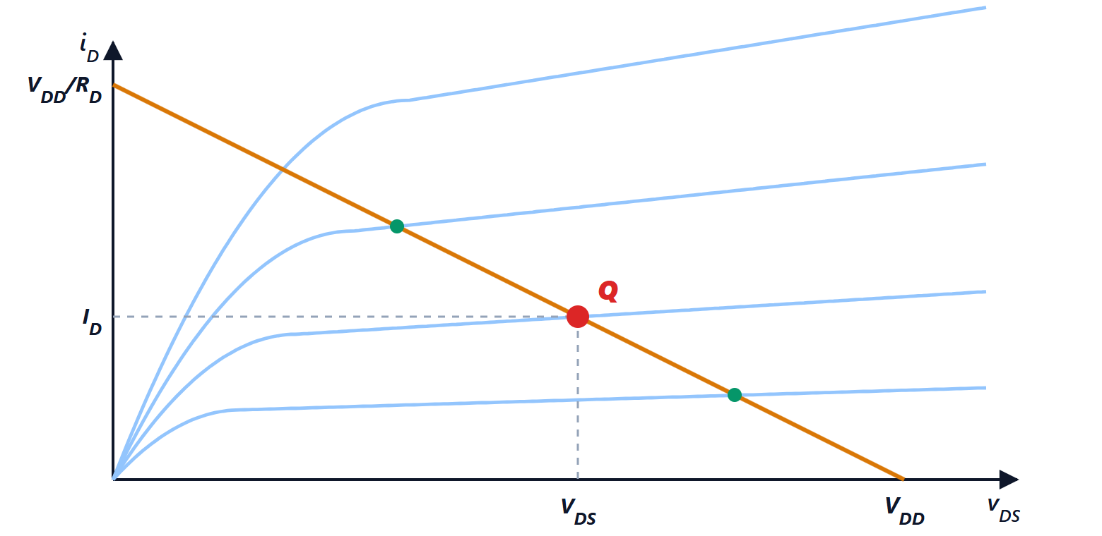
When the signal makes  swing, the point moves along the line: a small change in moves the point from one curve to another, and the projection on the
 axis shows a much larger change, of opposite sign. Q should be chosen in the middle of the useful range, away from both the triode region and cut-off, to leave room for the signal in both directions.
Transconductance
For small changes around Q, the characteristic can be replaced by its tangent. The key parameter is the transconductance, the derivative of the output current with respect to the input voltage:
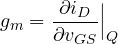
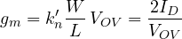
MOSFET. Differentiating the square law  :
BJT. Differentiating  :
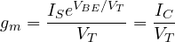
For the same current the BJT has a much higher transconductance: at 1 mA,  mA/V, while a MOSFET with
 V has 4 mA/V. On the other hand the BJT draws base current: seen from the base, its small-signal input resistance is
 , about 2.6 kΩ with
 and 1 mA.
The small-signal model
For signals only, the transistor is replaced by a linear circuit:
- a controlled current source
 (or
 ) between drain and source (collector and emitter);
- the output resistance
 in parallel, accounting for the Early effect or channel length modulation;
- for the BJT, the resistance
 between base and emitter.
For signals, DC supplies are short circuits to ground (their voltage does not change), and large coupling capacitors are short circuits at the signal frequency. The method is always the same: compute the DC bias, derive  , , , then analyse the linear small-signal circuit with the methods of Electrical Engineering.
How small. The tangent approximation holds as long as the input signal is small compared with the scale of the nonlinearity: for the BJT  , that is a few millivolts; for the MOSFET
 . Beyond that, the output distorts.
The common-source (or common-emitter) amplifier
Input at the gate, output at the drain, source grounded. With the small-signal model, the current  flows through the parallel combination of and :

The minus sign says the output is inverted: when the gate rises, the current grows, the drop across grows and the drain falls.
Examples. A MOSFET with  mA/V and
 kΩ:
 . A BJT at 1 mA with
 kΩ:
 . The largest gain achievable, with an ideal load, is
 , the transistor’s intrinsic gain:
 for the BJT, thousands; a few tens for modern short-channel MOSFETs.
If the bias circuit has an emitter (or source) resistor not bypassed by a capacitor, the gain drops to about  but becomes independent of the transistor and distortion decreases: an example of negative feedback.
The other configurations
| Configuration | Input / output | Voltage gain | Input resistance | Output resistance | Use |
|---|---|---|---|---|---|
| common source (emitter) | gate / drain | high, inverting | high (MOS) or medium (BJT) | high | gain stage |
| common drain (collector) | gate / source | about 1 | high | low, about  | buffer, output stage |
| common gate (base) | source / drain | high, non-inverting | low, about | high | high frequency, cascode |
The common-collector stage (emitter follower) does not amplify voltage, but “copies” it onto a heavy load: it is the typical output stage of audio amplifiers. Combining stages gives operational amplifiers, which have a differential input stage, one or two gain stages and an output stage.
Frequency limits
The transistor’s internal capacitances (gate-source and gate-drain, base-emitter and base-collector) reduce gain at high frequencies. In the common-source stage the capacitance between input and output appears at the input multiplied by about  (the Miller effect), and it is often what sets the bandwidth. The parameter that sums up a transistor’s speed is the transition frequency
 , at which the current gain drops to 1: tens or hundreds of gigahertz in current devices.