Radar propagation: multipath over the sea, refraction and ducting, rain attenuation, ionosphere

The radar equation of the first lesson assumes that the wave travels in a vacuum, in a straight line, without losses. In the real atmosphere, above a curved Earth that is often covered by water, things are different: the sea reflects the wave and creates multipath that reinforces or cancels the echo; the air bends the rays; rain and gases absorb energy; mountains and the horizon hide targets; the ionosphere reflects short waves. This lesson explains each of these effects and shows how they enter the radar equation through a single factor, the pattern propagation factor .

The idea in simple words

Think of someone talking on the shore of a calm lake: a listener on the other side receives two voices, the direct one and the one reflected by the water, which arrives with a small delay. Depending on the position, the two voices add up (louder sound) or cancel (almost no sound). Radio waves above the sea do exactly this, and the radar sees the target intermittently: strong at some ranges, invisible at others.

Then there is the air, which is not uniform: it is denser at low altitude, and waves travel slightly slower where the air is denser. As light does in a mirage, the ray bends downwards and the radar sees a little beyond the geometric horizon; sometimes, in particular conditions, much beyond. Finally rain: drops absorb and scatter the waves, more and more as the frequency increases.

The propagation factor

All effects enter the radar equation by multiplying the received power by and dividing by the atmospheric losses :

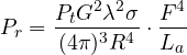
is the ratio between the field that actually reaches the target and the field that would reach it in free space; it appears to the fourth power because the path is travelled twice (out and back) and power is the square of the field. In free space .

Multipath over the sea

A radar at height and a target at height , at range much larger than the heights, above a flat and smooth surface (the calm sea, at low grazing angles, reflects almost everything with a coefficient of about ).

Theorem. Under these assumptions

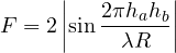
Proof. The direct ray travels ; the reflected one, by the method of images, behaves as if it started from a “mirrored” antenna at height , and travels . For , with , the path difference is . The total field is with : with . ∎

The consequences:

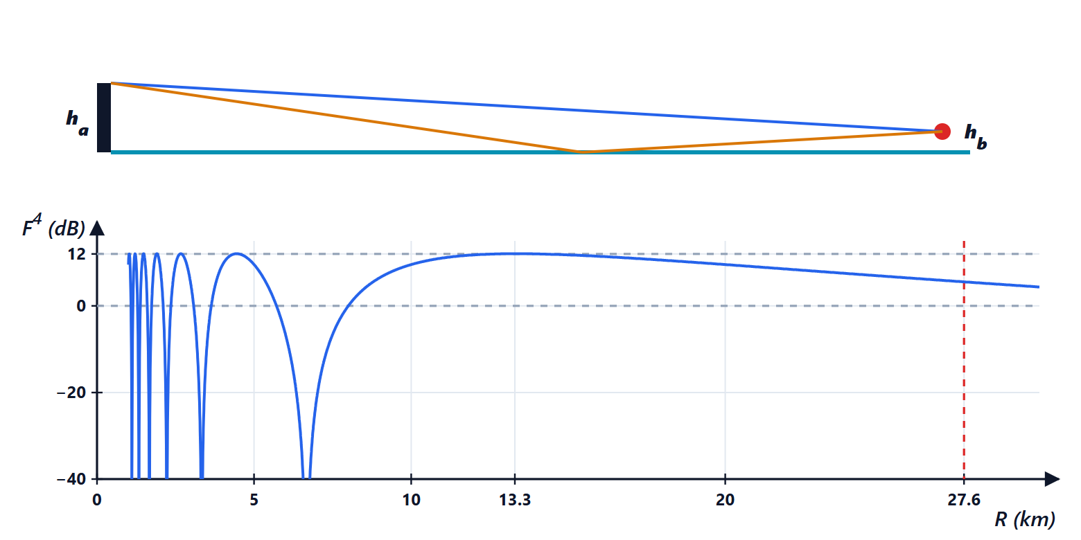
• oscillates between 0 and 2: where it is 2 the echo power is times (+12 dB) the free-space value; where it is 0 the target disappears. The vertical pattern of the antenna breaks into lobes.
• The last maximum is at ; beyond it the argument of the sine is small, , and the received power goes as 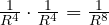: it falls much faster than in free space.

Example. X-band ship radar with the antenna at 20 m, anti-ship missile flying 5 m above the water. The last lobe is at 13 km (+12 dB); nulls at 6.7, 3.3, 2.2 km…; between 20 and 27 km the power falls by 8.9 dB, already close to the 10.4 dB of the law; and at 27.6 km is the radar horizon. This is why sea-skimming missiles are so hard to see: they appear late and intermittently.

In reality a rough sea reflects less (the reflection coefficient falls with roughness, Rayleigh criterion), and the curvature of the Earth reduces the effective heights and spreads the reflected ray: the nulls are less deep, but the phenomenon remains. It is countered by changing frequency (the lobes move), or by using antennas at several heights or different polarisations.

Refraction and the horizon

The refractive index of air is just above 1 (about 1.0003 at ground level) and is expressed through the refractivity , about 300 N units at sea level. In a “standard” atmosphere decreases with height by about 39 units per km. A ray crossing a medium whose index decreases upwards bends downwards, with radius of curvature .

The equivalent radius trick. Instead of drawing curved rays over a curved Earth, one draws straight rays over an Earth with a larger radius, , chosen so that the relative curvature stays the same: 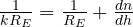, hence

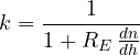
With N/km we get , the value used in the first lesson for the radar horizon .

Super-refraction and ducts. Above a warm sea, or with temperature inversions, the gradient can become much stronger: with −100 N/km, and the radar sees much farther than usual; at −157 N/km the curvature of the ray equals that of the Earth ( infinite): the wave is trapped in a duct and can travel hundreds of kilometres. The radar then sees very distant coasts as if they were close targets (with range ambiguities) and clutter increases. Conversely, in sub-refraction the horizon shrinks and shadow zones appear.

Diffraction. Beyond the horizon or behind a mountain the wave does not stop abruptly: a small part arrives by diffraction (like sound around a corner), but it decreases quickly, the more so the higher the frequency. Low frequencies (VHF, UHF) “bend” better around obstacles.

Atmospheric absorption and rain

Gases. Oxygen and water vapour absorb microwaves, with absorption lines at 22 GHz (vapour), 60 GHz and 119 GHz (oxygen). Below 10 GHz the clear-air absorption is small (in X band about 0.01 dB/km one way); at 60 GHz it is about 15 dB/km, so strong that this band is used for very short range communications that must not disturb farther away. The 77 GHz car radar sits in a “window” between the lines.

Rain. The specific attenuation of rain is expressed as dB/km, with the rain rate in mm/h and , tabulated as functions of frequency (ITU-R Recommendation P.838). In X band (, ): 0.09 dB/km for light rain of 5 mm/h, 0.70 dB/km for 25 mm/h, 1.66 dB/km for a 50 mm/h thunderstorm. Crossing 10 km of thunderstorm, out and back, 33 dB are lost: the target behind the storm disappears. In S band the attenuation is tens of times smaller: this is why long-range surveillance radars and large weather radars work at low frequencies, while high-frequency radars are used where distances are short. Rain, besides attenuating, reflects: it is the volume clutter of the lesson on clutter, and it is the useful signal of weather radars.

The ionosphere and over-the-horizon radars

Above 80 km the ionosphere, a layer of ionised gas, reflects short waves (HF, 3-30 MHz). Over-the-horizon (OTH) radars exploit this natural mirror: the wave goes up, is reflected, comes down 1000-3000 km away and illuminates aircraft and ships far beyond the horizon. Performance depends on the time of day, the season and solar activity, which change the height and density of the ionosphere, and resolution is poor (low frequencies, little bandwidth); but coverage is huge. At higher frequencies the ionosphere is crossed, with smaller effects: delays and rotation of the polarisation (Faraday rotation, seen in the Electromagnetic Fields course), important for space radars and for L- and P-band SARs.

Summary

• Propagation effects enter the radar equation as .
• Above a reflecting surface (the sea) the direct and reflected rays interfere: lobes up to +12 dB and nulls, then a decay as at low angles. Low targets are seen late.
• Refraction bends rays downwards: the equivalent Earth radius is used; with strong gradients ducts form and the radar sees very far.
• Gases and rain attenuate, more and more as frequency increases: S and L bands for long ranges, X band and above for short ones.
• The ionosphere reflects short waves and makes over-the-horizon radars possible.

The code

import numpy as np

c = 299792458.0
f = 10e9; lam = c / f                                  # X band
ha, hb = 20.0, 5.0                                     # ship antenna at 20 m, missile 5 m above the sea

# 1) multipath over a flat reflecting surface (coefficient -1): propagation factor F
print(f"last maximum (F = 2, +12 dB in power) at {4 * ha * hb / lam / 1e3:.0f} km")
print("nulls at", ", ".join(f"{2 * ha * hb / (lam * k) / 1e3:.1f}" for k in (1, 2, 3)), "km")
RE = 6371e3
horizon = np.sqrt(2 * 4 / 3 * RE * ha) + np.sqrt(2 * 4 / 3 * RE * hb)
print(f"radar horizon for this geometry: {horizon / 1e3:.1f} km")
for Rk in (13.3e3, 20e3, 27e3):
    Fk = 2 * abs(np.sin(2 * np.pi * ha * hb / (lam * Rk)))
    print(f"at {Rk / 1e3:.0f} km: F^4 = {40 * np.log10(Fk):.1f} dB (free space = 0 dB)")
Rl = np.array([20e3, 27e3])
F4 = 40 * np.log10(2 * np.abs(np.sin(2 * np.pi * ha * hb / (lam * Rl))))
print(f"from 20 to 27 km: F^4 falls by {F4[0] - F4[1]:.1f} dB, free space (R^-4) by {40 * np.log10(27 / 20):.1f} dB; in total {F4[0] - F4[1] + 40 * np.log10(27 / 20):.1f} dB, R^-8 would give {80 * np.log10(27 / 20):.1f} dB")

# 2) refraction: equivalent Earth radius from the refractivity gradient N = (n - 1) 1e6
for dN in (-39, -100, -157):                           # N units per km
    den = 1 + RE * dN * 1e-9
    k = 1 / den if den > 0 else np.inf
    print(f"dN/dh = {dN:4d} N/km: k = {k:.2f}" + ("  (duct: the ray follows the Earth)" if den <= 0 else ""))

# 3) rain attenuation in X band: gamma = k R^alpha (ITU-R P.838, 10 GHz, horizontal polarisation)
kp, alpha = 0.01217, 1.2571
for rain in (5, 25, 50):
    g = kp * rain ** alpha
    print(f"rain {rain:2d} mm/h: {g:.2f} dB/km, out and back through 10 km of rain {2 * 10 * g:.1f} dB")

Running it prints 13 km for the last lobe, the nulls at 6.7, 3.3 and 2.2 km, the horizon at 27.6 km, of 12.0, 9.5 and 5.9 dB at 13, 20 and 27 km, the 8.9 dB decrease against the 10.4 dB of the law, and 2.76 and the duct at −157 N/km, and 1.8, 13.9 and 33.3 dB of attenuation in the three rain cases.