CPU scheduling: FCFS, SJF, round robin and the Linux scheduler
Performance measures, optimality of SJF proved by exchange, exponential averaging of bursts, the round-robin waiting bound proved, multilevel queues, CFS.
When several processes are ready, the scheduler decides who uses the CPU and for how long. The possible choices favour different goals: finishing many jobs, responding quickly to the user, being fair, meeting deadlines. In this lesson we look at performance measures, the classic algorithms with the proof that “shortest first” minimises average waiting, duration estimation, round robin with its bound on response time, priorities and the Linux scheduler.
The measures
For each process we measure:
- the turnaround time: from arrival to completion;
- the waiting time: the time spent ready in the queue, without running;
- the response time: from arrival to first execution, important for interactive programs.
For the system what counts is throughput, the number of jobs completed per unit time, and CPU utilisation. Processes alternate bursts of computation (CPU bursts) and input/output waits: interactive processes have short bursts, compute-bound ones long bursts.
FCFS and SJF
FCFS (first come, first served) runs processes in order of arrival. It is simple but suffers from the convoy effect: one long job in front makes all the short ones behind it wait. SJF (shortest job first) runs the job with the shortest burst first.
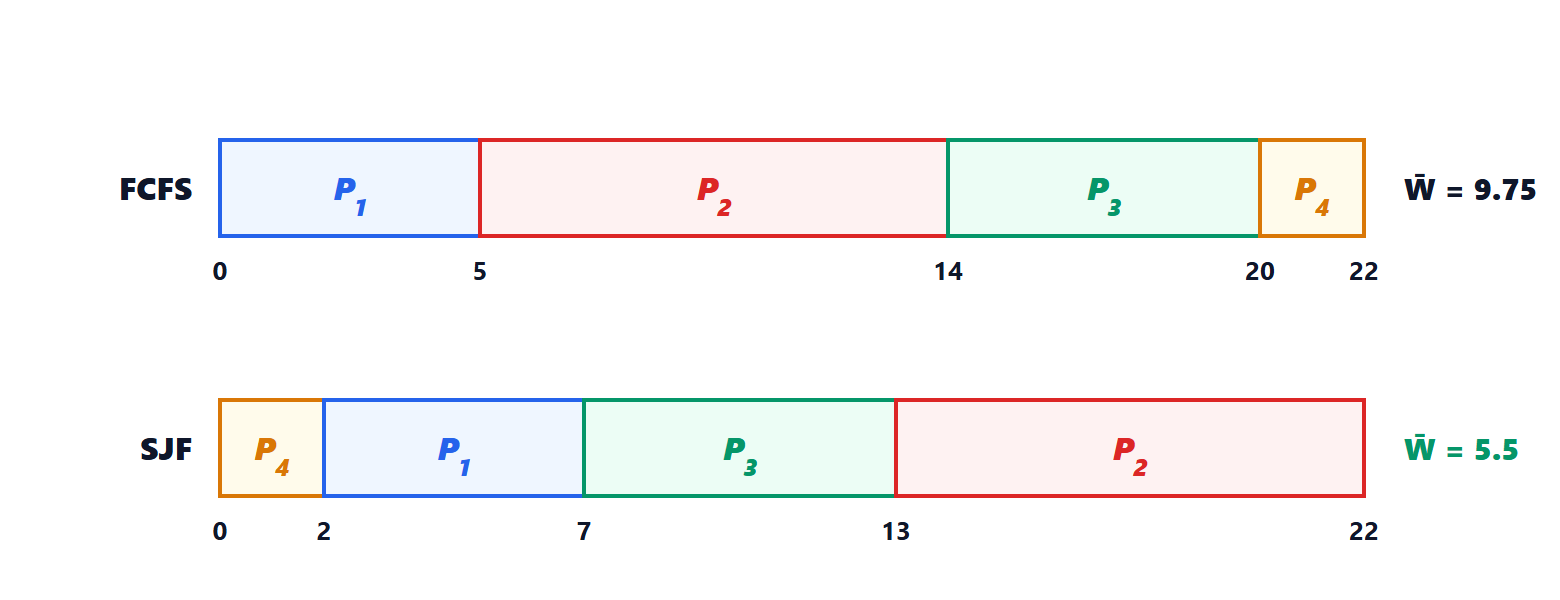
Example. With FCFS the waiting times are 0, 5, 14, 20, average 9.75; with SJF they are 0 (P4), 2 (P1), 7 (P3), 13 (P2), average 5.5.
Theorem. Among all non-preemptive orderings of  jobs available at time 0, SJF minimises the average waiting time.
Proof (exchange). Consider an ordering in which two consecutive jobs  and
 have durations
 , with before . Swapping them, the waiting time of the earlier and later jobs does not change (the later ones wait
 for the two anyway). The waiting time of decreases by
 and that of increases by
 : the sum decreases by
 . So every ordering with a consecutive “long before short” pair can be improved, and the optimum has none: it is the ordering by increasing duration, i.e. SJF. ∎
The same exchange argument proves many optimality results in scheduling (Business Management lesson on production scheduling).
Estimating the future
SJF requires knowing the duration of the next burst, which is unknown. It is estimated with an exponential average of past bursts:

where  is the measured duration of the last burst and
 the weight of recent history. It is a first-order low-pass filter (lesson on discrete-time systems). The preemptive version, SRTF (shortest remaining time first), interrupts the running process if one arrives with a burst shorter than its remaining time. The risk of both is starvation of long jobs, if short jobs keep arriving.
Round robin
Round robin gives every ready process, in turn, a time quantum  ; when it expires the process goes back to the end of the queue (the transition from running to ready in the state diagram, lesson on processes).
Theorem. With ready processes and quantum , no process waits more than  before its turn.
Proof. In front of a process in the queue there are at most  processes, and each uses the CPU for at most before being put back at the end. ∎
The quantum is a trade-off. If is large, round robin becomes FCFS; if it is small, response is fast but the context switch, lasting  , weighs: the useful fraction of time is
 . With
 µs and
 ms the cost is 0.1 %; with
 µs it would be almost 10 %. Usually the quantum is chosen longer than the typical burst of interactive processes, which thus finish before it expires.
Priorities and multiple queues
Real schedulers assign priorities: interactive or system processes before compute-bound ones. To avoid starvation of low-priority processes aging is used: priority grows with the time spent waiting.
The multilevel feedback queue (MLFQ) learns the nature of processes without knowing it in advance: a new process enters the highest-priority queue with a short quantum; if it uses its whole quantum it moves down a level, if it blocks earlier it stays up. Interactive processes thus stay at the top, compute-bound ones move down to queues with longer quanta.
The Linux scheduler
The Linux scheduler for ordinary processes, CFS (completely fair scheduler, replaced from version 6.6 by its evolution EEVDF with the same principle), tries to give each process a fair share of the CPU. It keeps for each process a virtual runtime, which grows while the process runs, more slowly for more important processes; it always runs the process with the minimum virtual runtime, keeping processes in a balanced binary tree. A process that sleeps a lot (interactive) accumulates little virtual runtime and, when it wakes up, runs immediately. Importance is set with the “nice” value: each step changes the weight by about 25 %.
On multiprocessor systems the scheduler must also balance the load across cores and, on the contrary, keep a process on the same core (affinity) to exploit the caches already filled with its data. Real-time processes need different rules, with guaranteed deadlines (lesson on real-time systems).





