Structural safety: limit states, reliability and partial factors
Ultimate and serviceability limit states, reliability index and failure probability proved with an example, characteristic values, partial factors and load combination with an example.
Building techniques (structural design) apply structural mechanics to real design: with real materials, uncertain loads, codes to comply with. The first question is what “safe” means: loads and resistances are not exact numbers but random variables, and zero risk does not exist. In this lesson we look at limit states, the reliability index with the proof of the failure probability and an example, characteristic values with an example, and the partial factor method of the codes, with a load combination.
Limit states
A limit state is a condition beyond which the structure no longer satisfies a requirement:
- ultimate limit states (ULS): collapse, rupture of a section, instability, overturning, loss of equilibrium; they concern people’s safety;
- serviceability limit states (SLS): excessive deflections (Structural Mechanics lesson on the elastic line), cracking, annoying vibrations; they concern functionality and durability.
The European codes (Eurocodes) and the Italian ones (Norme tecniche per le costruzioni, NTC 2018) require both to be checked.
Reliability
Let  be the resistance of an element and
 the effect of the actions on it (the same kind of quantity: two forces, two moments). Failure occurs if
 .
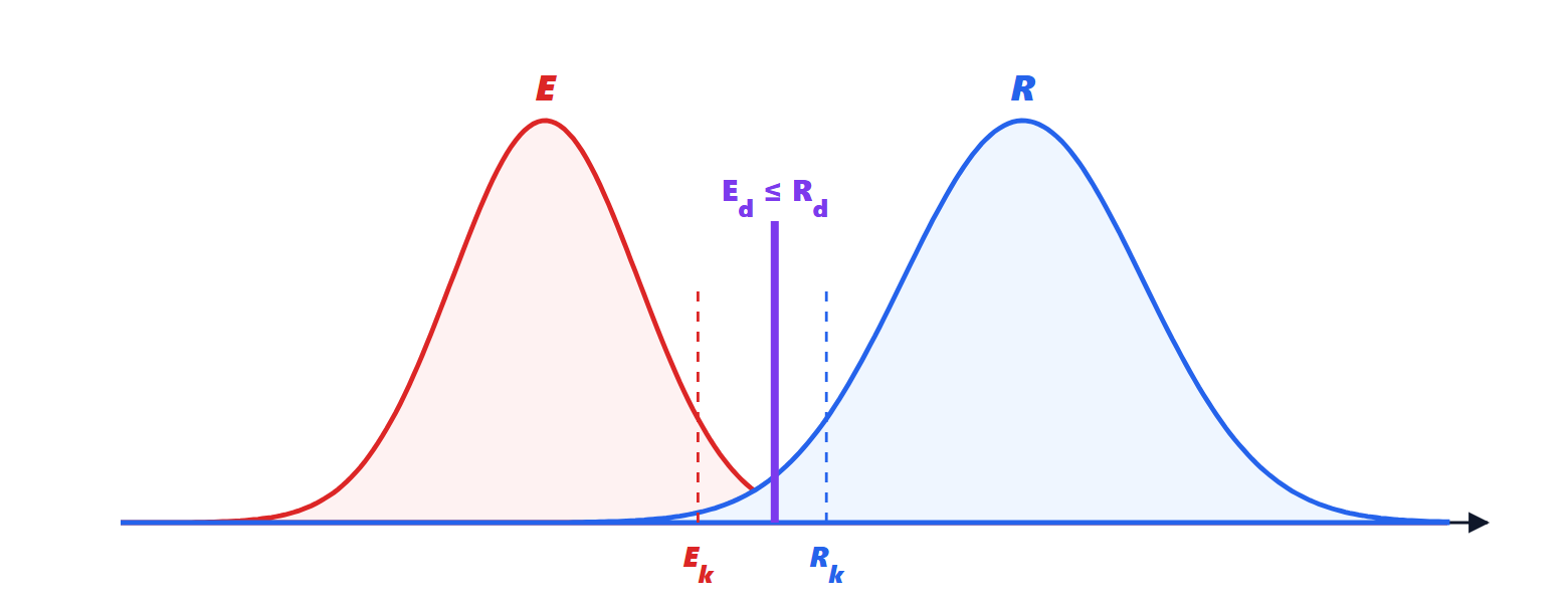
Theorem. If and are independent Gaussians, the failure probability is

where  is the standard normal distribution function and
 the reliability index.
Proof. The margin  is Gaussian, as a difference of independent Gaussians, with mean
 and variance
 (Signal Theory lesson on probability). Failure is the event
 , whose probability, standardising, is
 . ∎
Example. With  ,
 ,
 ,
 (in any units):
 ,
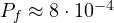 . European codes aim, for ordinary buildings, at
 over 50 years, i.e.
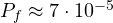 . Safety depends not only on the ratio of the means but also on the scatter: a very variable material requires a larger margin.
Characteristic values
Full probabilistic calculation is reserved for special cases; in practice representative values are used. The characteristic value of a resistance is the 5 % fractile: the value that only 5 % of samples fail to reach. For a normal distribution

because  . Example. Concrete cubes with a mean strength of 38 MPa and a standard deviation of 4 MPa:
 MPa. For actions, the characteristic value is instead an upper fractile (for variable loads, usually the one with a 50-year return period).
The partial factor method
Codes transform the probabilistic problem into a deterministic check: design values are compared, obtained by dividing characteristic resistances by factors  and multiplying characteristic actions by factors
 :

The factors are calibrated so that the check corresponds to the target reliability. Typical values: for concrete  , for reinforcing steel
 , for structural steel
 ; for structural permanent loads
 , for non-structural ones and variable loads
 . The more uncertain a quantity, the larger its factor.
When several variable loads act, they are unlikely to reach their characteristic values together: one is taken as leading, the others are reduced by combination factors  . The fundamental ULS combination is

Example. A floor with self-weight  kN/m², finishes and partitions
 kN/m², residential imposed load
 kN/m². At ULS:
 kN/m². For serviceability checks combinations without amplification factors are used: the characteristic combination gives
 kN/m². If a permanent load is favourable (for example the weight stabilising a wall against overturning), a factor less than 1 is used: safety requires considering the most unfavourable situation in every check.