PERT and CPM: activity network, critical path proved, probability of finishing on time and crashing at minimum cost
Project scheduling with PERT and CPM on a complete example: forward and backward pass, slack and critical path with proof, three estimates and probability of meeting the deadline, Monte Carlo check of PERT's optimism, crashing at minimum cost, Python code.
https://www.electronics-engineering.com/en/pert-cpm-critical-path-project-scheduling-monte-carlo-crashing/
A project (developing a product, building a plant, organising an event) is made of activities linked by precedence constraints: assembling the prototype cannot start before the components arrive. The PERT (Program Evaluation and Review Technique) and CPM (Critical Path Method) methods, both born at the end of the 1950s, answer three questions: how long the project lasts, which activities cannot be delayed without delaying everything, and how likely we are to finish by a given date. CPM, developed by DuPont for chemical plant maintenance, uses fixed durations and also considers costs; PERT, devised for the US Navy’s Polaris missile programme, treats durations as random variables. This lesson derives them step by step on an example, checks PERT with a simulation and shows how to shorten a project at minimum cost.
The idea in simple words
Think of a dinner: the pasta cooks while you prepare the sauce, but you can drain it only when both are ready. The total time is not the sum of everything, but the longest sequence of things that must happen one after the other: the critical path. The activities on that path are the ones that, if late, make the dinner late; the others have some slack (the sauce can wait). PERT and CPM carry out this reasoning systematically for projects with tens or thousands of activities.
The activity network
Each activity has a duration and a list of predecessors. The project is represented as a directed acyclic graph: the nodes are the activities, the arrows the “must finish before” constraints. (There is also the activity-on-arrow representation of the classic PERT textbooks; activity-on-node is the most used today.)
The example of this lesson is the development of a small electronic product, with durations in weeks:
| activity | description | predecessors | a | m | b | expected duration |
|---|---|---|---|---|---|---|
| A | specifications | none | 2 | 3 | 5 | 3.17 |
| B | hardware design | A | 4 | 6 | 10 | 6.33 |
| C | software design | A | 5 | 8 | 14 | 8.50 |
| D | component purchasing | B | 3 | 4 | 8 | 4.50 |
| E | prototype assembly | D | 2 | 3 | 5 | 3.17 |
| F | software testing | C | 2 | 4 | 6 | 4.00 |
| G | integration | E, F | 3 | 5 | 9 | 5.33 |
| H | certification | G | 3 | 4 | 7 | 4.33 |
The three columns a, m, b are the optimistic, most likely and pessimistic PERT estimates; for now the expected duration  is enough, and it is discussed further on.
The two passes and the critical path
Forward pass. Following the graph from the start, each activity can begin at the earliest when all its predecessors have finished:

The project duration is  .
Backward pass. Starting from the end, each activity must finish at the latest when the first of its successors must start, without moving the end date  :

The slack (total float) of an activity is  : how much it can slip without delaying the project. The activities with zero slack form the critical path.
Theorem. The minimum project duration is the length of the longest path from the start to the end of the graph, and the forward pass computes it.
Proof. Along any path the activities must take place one after the other, so the project cannot last less than the sum of their durations:  the length of every path, in particular the longest. Conversely, by induction on the topological order,
 is exactly the length of the longest path ending in
 : it holds for the initial activities, and if it holds for all predecessors of , then
 is the longest path reaching and the one ending with . Starting each activity at its
 satisfies all constraints and finishes at
 : the minimum duration is achieved. ∎
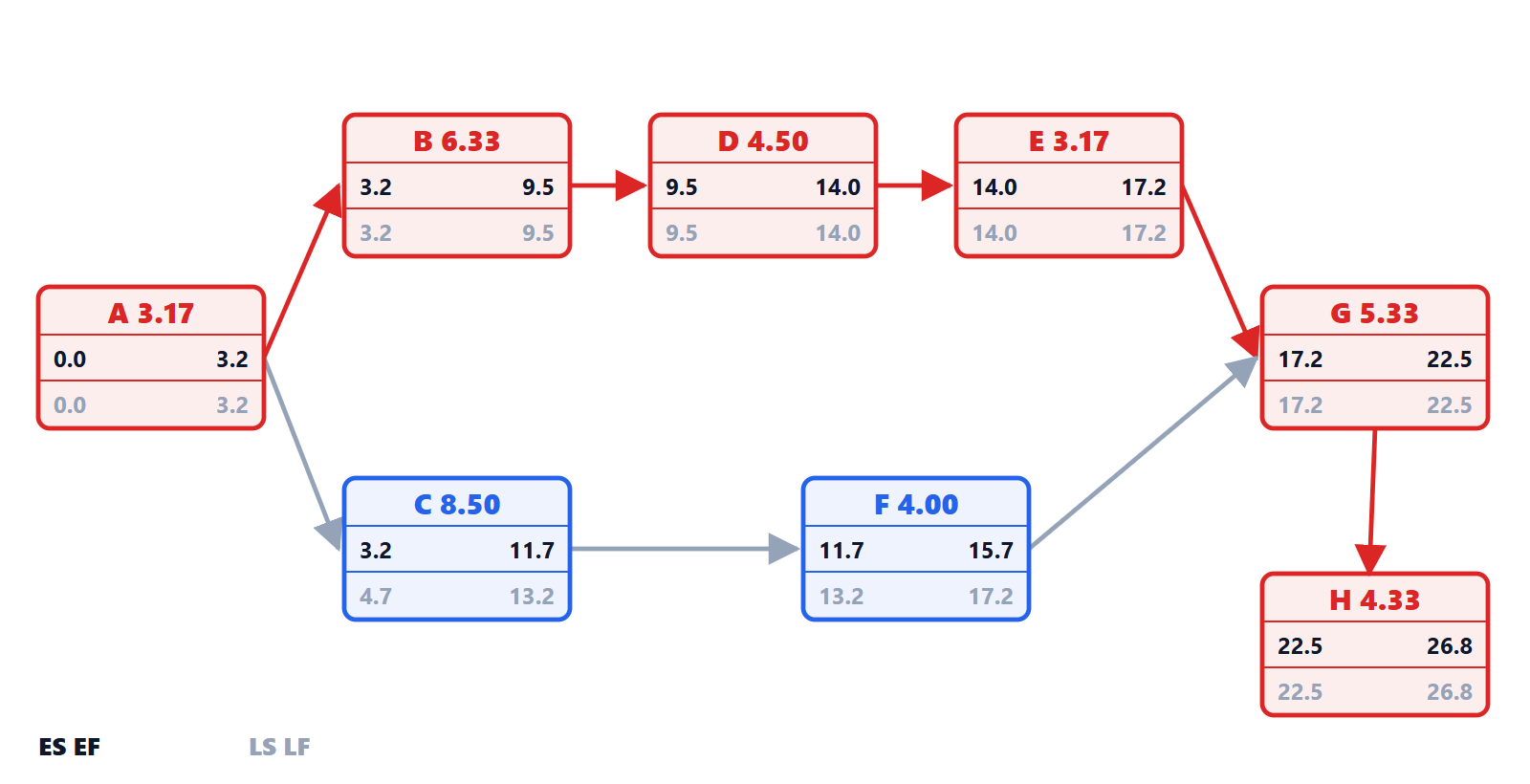
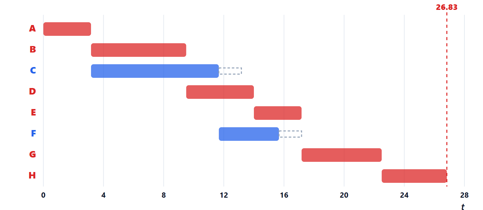
In the example, with the expected durations: the project lasts 26.83 weeks and the critical path is A-B-D-E-G-H (hardware design, purchasing, assembly, integration, certification). The software branch, C-F, has a slack of 1.5 weeks: it can slip by up to a week and a half with no consequence.
PERT: uncertain durations
In PERT each duration is a random variable described by three estimates: optimistic  , most likely
 , pessimistic
 . It is assumed to follow a beta distribution on
 with mode , and the classic approximations are used

(the mean weighs the most likely estimate four times; the standard deviation is one sixth of the range, as for a normal distribution in which almost all values lie within ±3σ).
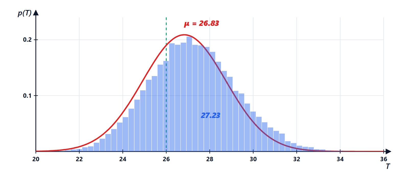
PERT then computes the critical path with the expected durations and approximates the project duration as the sum of the durations of the critical activities, which by the central limit theorem is roughly normal, with mean the sum of the means and variance the sum of the variances (independent activities). In the example  weeks, and the probability of finishing within 26 weeks is

PERT is optimistic. The method looks at a single path, but the project finishes when all paths finish: if the software activities run long, the C-F branch can become critical too. The maximum of several random variables has a mean larger than the maximum of the means (Jensen’s inequality applied to the maximum, which is a convex function). A Monte Carlo simulation of 200 000 projects, each with durations drawn from their beta distributions, gives a mean duration of 27.23 weeks instead of 26.83 and a probability of finishing within 26 weeks of 27.8 % instead of 33.1 %. This is the so-called merge bias: in projects with many nearly critical parallel branches the PERT error can be much larger, and simulation is the right tool.
CPM: shortening at minimum cost
CPM adds costs. Many activities can be shortened (crashing) by paying more: overtime, express shipping, more people. For each activity one knows how much it can be reduced and what each saved week costs. The problem is: how to reduce the project duration by a given amount while spending as little as possible?
The rules that follow:
- only critical activities are worth shortening: shortening an activity with slack does not change the duration;
- among the critical ones, the one with the lowest cost per week is chosen;
- when another path becomes critical, both must be shortened, and activities shared by the two paths become attractive.
In the example, with the most likely durations the project lasts 25 weeks: path A-B-D-E-G-H is 25 long, path A-C-F-G-H 24. To get down to 23 weeks, 2 weeks must be taken off the first and 1 off the second. The optimal solution, found by the code by trying every combination, is to shorten G (shared by both paths, 2000 euros) and E (1500 euros): 3500 euros. Shortening only activities of the first path, for example E and B, would not be enough: the second path would remain at 24 weeks. Large projects are solved with linear programming.
Summary
- The project is a graph of activities with precedences; its minimum duration is the longest path.
- The forward pass gives the earliest starts, the backward pass the latest starts; slack is the difference, and the activities without slack form the critical path.
- PERT uses three estimates per activity,
 and
 , and approximates the duration with a normal distribution on the critical path.
- PERT is optimistic when several paths are nearly critical: Monte Carlo simulation gives the correct estimate.
- CPM shortens the cheapest critical activities, taking into account the paths that become critical.
The original notes on this topic, from the Operations Research course, are in the web archive: notes on PERT (PDF, Italian).
The code
import itertools
import math
import numpy as np

# Project of a small electronic product: activities, precedences and three estimates (optimistic, most likely, pessimistic), in weeks
act = {
    "A": ((2, 3, 5), []),             # specifications
    "B": ((4, 6, 10), ["A"]),         # hardware design
    "C": ((5, 8, 14), ["A"]),         # software design
    "D": ((3, 4, 8), ["B"]),          # component purchasing
    "E": ((2, 3, 5), ["D"]),          # prototype assembly
    "F": ((2, 4, 6), ["C"]),          # software testing
    "G": ((3, 5, 9), ["E", "F"]),     # integration
    "H": ((3, 4, 7), ["G"]),          # certification
}
te = {k: (a + 4 * m + b) / 6 for k, ((a, m, b), _) in act.items()}       # PERT expected duration
var = {k: ((b - a) / 6) ** 2 for k, ((a, m, b), _) in act.items()}       # PERT variance
order = list(act)                                                        # already in topological order

def cpm(dur):
    ES, EF = {}, {}
    for k in order:                                                      # forward pass
        ES[k] = max((EF[p] for p in act[k][1]), default=0.0)
        EF[k] = ES[k] + dur[k]
    T = max(EF.values())
    LF, LS = {}, {}
    for k in reversed(order):                                            # backward pass
        succ = [s for s in order if k in act[s][1]]
        LF[k] = min((LS[s] for s in succ), default=T)
        LS[k] = LF[k] - dur[k]
    return T, ES, EF, LS, LF

T, ES, EF, LS, LF = cpm(te)
crit = [k for k in order if abs(LS[k] - ES[k]) < 1e-9]
print(f"expected project duration {T:.2f} weeks, critical path {'-'.join(crit)}")
for k in order:
    print(f"  {k}: te {te[k]:.2f}  ES {ES[k]:5.2f}  EF {EF[k]:5.2f}  LS {LS[k]:5.2f}  LF {LF[k]:5.2f}  slack {LS[k] - ES[k]:.2f}")

# probability of finishing within 26 weeks according to PERT (sum of the variances on the critical path, normal distribution)
s = math.sqrt(sum(var[k] for k in crit))
Phi = lambda z: 0.5 * (1 + math.erf(z / math.sqrt(2)))
print(f"PERT: sigma {s:.2f} weeks, P(T <= 26) = {Phi((26 - T) / s):.3f}")

# Monte Carlo check with beta-PERT distributed durations
rng = np.random.default_rng(0)
N = 200_000
samp = {}
for k, ((a, m, b), _) in act.items():
    al, be = 1 + 4 * (m - a) / (b - a), 1 + 4 * (b - m) / (b - a)
    samp[k] = a + (b - a) * rng.beta(al, be, N)
EFs = {}
for k in order:
    EFs[k] = np.max([EFs[p] for p in act[k][1]], axis=0) + samp[k] if act[k][1] else samp[k]
Tmc = EFs["H"]
print(f"Monte Carlo: mean duration {Tmc.mean():.2f}, P(T <= 26) = {np.mean(Tmc <= 26):.3f}")

# CPM: shorten the project by 2 weeks at minimum cost (maximum reduction and cost per week of each activity)
norm = {k: act[k][0][1] for k in order}                                  # most likely durations m
crash = {"A": (1, 3000), "B": (2, 2500), "C": (2, 1800), "D": (1, 4000), "E": (1, 1500), "F": (1, 1200), "G": (2, 2000), "H": (1, 5000)}
T0 = cpm(norm)[0]
best = None
for red in itertools.product(*[range(crash[k][0] + 1) for k in order]):
    dur = {k: norm[k] - r for k, r in zip(order, red)}
    if cpm(dur)[0] <= T0 - 2:
        cost = sum(r * crash[k][1] for k, r in zip(order, red))
        if best is None or cost < best[0]:
            best = (cost, {k: r for k, r in zip(order, red) if r})
print(f"duration with the most likely durations {T0:.0f} weeks; to reach {T0 - 2:.0f}: reductions {best[1]}, cost {best[0]} euros")
Running it prints the expected duration of 26.83 weeks with the critical path A-B-D-E-G-H and the table of the two passes (slack 1.50 for C and F), σ = 1.91 and probability 0.331 according to PERT, mean duration 27.23 and probability 0.278 in the simulation, and for CPM the reductions of E and G at a cost of 3500 euros.





Ciao, sono l'autore di «PERT e CPM: reticolo delle attività, cammino critico dimostrato, probabilità di finire in tempo e accelerazione al costo minimo». Domande, dubbi, segnalazioni di errori o richieste di approfondimento sono benvenuti: scriveteli qui sotto e vi rispondo io. Potete anche votare la pagina con le stelle all'inizio dell'articolo.Hi, I am the author of “PERT and CPM: activity network, critical path proved, probability of finishing on time and crashing at minimum cost”. Questions, doubts, error reports and requests for more detail are all welcome: write them below and I will answer. You can also rate the page with the stars at the top of the article.