Assembler and Simulator for the 6502 Processor Built in Visual Basic
Introduction. Aim of the course. This course aims to guide students in building an assembler and a simulator for a microprocessor of their choice, using a programming language…
https://www.electronics-engineering.com/en/assembler-and-simulator-for-the-6502-processor-built-in-visual-basic/
Introduction
Aim of the course. This course aims to guide students in building an assembler and a simulator for a microprocessor of their choice, using a programming language. This challenge will require the design of a complex program, which will let you deepen your skills in the chosen language. Even if some hardware features, such as interrupts, may not be fully simulated in the program, at the end of the course students will have gained a solid understanding of how an assembler and a simulator work.
The choice of language
Choice of language. For this project we selected the Visual Basic programming language. This language runs in the Windows environment and offers considerable advantages, especially in graphics and table creation, compared with other languages used in the MS-DOS environment. Even so, the instructions used do not differ significantly from those of other languages. One of the main features of Visual languages is their structure, which is based on handling graphical features and on dividing the code into subroutines. These subroutines are not called by a main program, but by events triggered by graphical controls provided by VB, such as buttons and status bars. We chose this language for its excellent capabilities in handling tables and graphics, two fundamental aspects of this project.
The type of processor
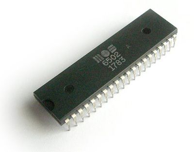
Type of microprocessor. The microprocessor selected for this project is the 6502. This microprocessor has a 16-bit address bus, allowing access to 64 Kbytes of memory. It also has an 8-bit data bus and 8-bit internal registers. This configuration means that, to work with data of 16 bits or more, the problem must be tackled in software, which results in longer execution times than microprocessors with larger data buses and registers.
Assembler
Assembler. The program was designed to create an assembler similar to a real one, without making significant changes to simplify the writing of the program in Visual Basic. This choice makes it possible to use assembly programs already developed without having to adapt them further. However, the main disadvantage of this approach is that the assembly program runs more slowly, because the listing of the assembly program must be traversed at least three times to obtain the desired result.
Now let us describe the graphical interface that will be presented to the user:
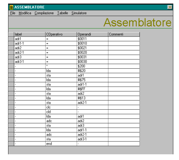
In this program, assembly language is not written in a traditional text editor, but inside a grid similar to an MS-Excel worksheet. This grid is an object made available by VB (DBGrid) and its job is to represent a database in the form of a table. Basically, when we write our program inside this table, we are actually populating a database in memory.
Now we must assess whether this choice is better than using a traditional text editor. With a text editor, the program would have to be saved in a file, which would then be read by the assembler. This would have meant opening and closing the file for every instruction, slowing the execution of the program considerably.
In our approach the database is always in memory, which means reading times for the database cells are considerably faster than opening a file previously written with a text editor. Our method also offers a better graphical appearance, which makes the assembly program easier to write and understand. This choice was made possible by the use of VB.
Once the program is written, it can easily be saved to a file with the extension .ASS. In this way you can clear the whole content of the database to create a new program or open another previously created .ASS file. This ability to handle sequential files is a feature provided by VB.
At this point, to obtain the output of the assembler, the compilation phase must be run, which is essentially the whole assembler process. During this phase the symbol table and the listing table, which are the results of assembly, are populated. It is important to note that this phase requires three passes of the assembly program created:
- In the first pass:
- The labels of the assembly program are entered in the label column of the symbol table, which was already defined earlier as a static table.
- It is determined whether each label in the symbol table represents a variable or a flag.
- It is identified whether the variable is in page 0 or not. This information is obtained from the addresses assigned to the variables in the assembly program.
- The MACHINE1 value of all the operation codes (opcodes) of all the lines is looked up and entered in a temporary table called the “intermediate table”.
- In this intermediate table, the type values that characterise the parts of the opcodes with a specific addressing mode are assigned.
- The addressing type is determined using letters of the alphabet in a specific order, based on the form in which the operand is written in the assembly program.
- Knowing the addressing type, the length of the instruction can be calculated and the code address incremented accordingly. This information is recorded in the intermediate table.
- Using the addressing and the type value, the value of MACHINE1PLUS can be calculated. The hexadecimal sum of MACHINE1 and MACHINE1PLUS is the machine code that identifies the opcode with a given addressing mode.
- In the second pass:
- The addresses corresponding to the labels are entered in the symbol table, using the information previously entered in the intermediate table during the first pass.
- In the third pass:
- The value of the operand is looked up in the symbol table, which is present in the assembly program.
- The listing table is completely filled in with the necessary information, whose structure was already defined earlier.
The next three figures show the symbol table, the intermediate table and the listing table.

The assembler can also create the listing file, with extension .LIS, and the numeric file, with extension .NUM. Once the numeric file has been created you can access the simulator. Before that you cannot,
because our simulator takes its data from the numeric file.
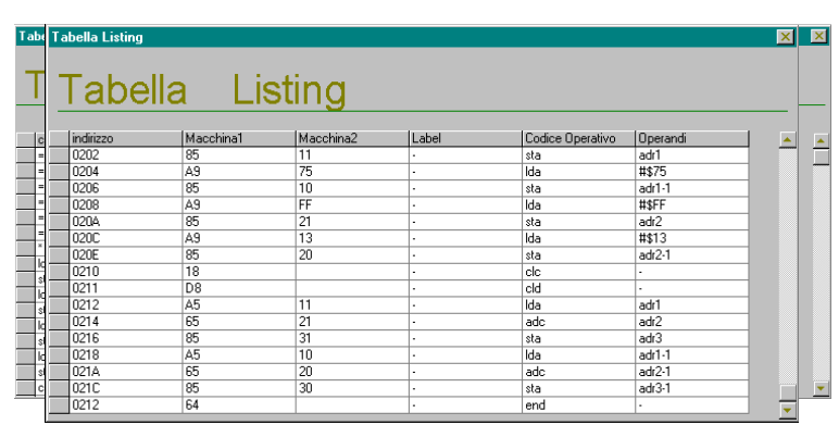
The listing file is a file that can be read by any text editor; its form is the following

The numeric file is built with a one-to-one correspondence, that is if the instruction is three bytes long then three bytes are transferred to the file.
The file format is a binary file (a VB feature) and the integer values of each hexadecimal byte of the code are written inside it.
The simulator that we shall now discuss takes its data from this numeric file
The simulator
The first operation performed by the simulator is to read the bytes from the numeric file and store them in the simulator memory. The simulator memory is represented by a 255×255 matrix, in which each row corresponds to a page of memory. The first row therefore represents page 0.
The program is loaded into memory starting from the location indicated by the first instruction in the numeric file. For example, considering the content of the listing file shown earlier, the first instruction is “FF 0020”. This instruction indicates that the numeric file must be written into the simulator memory starting from location 0200.
The program may contain subroutines, and in that case they must be preceded by an instruction of the type “FF __” that indicates the point in memory at which to start writing the subroutine. The main program must be written after all the subroutines.
Once the bytes have been loaded into memory, the Program Counter (PC) automatically points to the start of the location indicated by the first instruction of the main program.
The simulator must now execute the instructions, and to do so it must recognise each instruction of the program. To achieve this, a procedure must be associated with each machine code that represents an opcode.
To handle this, a “CASE” control structure can be used which, according to the machine code present, determines the addressing type and the operation to perform. However, this solution may not be the most efficient, because it could involve more than 150 branches in the “CASE”, making execution slow.
Instead, the solution adopted is to use a table that lists all the possible machine codes, together with their opcodes and addressing types. When a machine code is looked up, the corresponding addressing type and opcode are also found in the table.
Once the addressing type is known, a second “CASE” with 8 branches can be used to determine the data needed for the operations. Then a third “CASE” with 59 branches is used to determine the specific operation to perform for each opcode, using the data obtained from the addressing “CASE”.
This solution is more efficient, and the speed of looking up the machine code in the table can be improved further by assigning an index to the machine-code fields in the table, so as to order them in memory.
Finally, the addressing “CASE” determines the data, increments the PC appropriately and fetches the operand of each machine instruction (MACHINE2). Execution of the program continues until the “END” instruction is reached, which marks the last instruction to be processed by the simulator.

Now let us describe how the simulator is displayed graphically:
As shown in the previous form, the internal registers and the system flags can easily be identified. It is also easy to observe the results in the respective memory locations in the “on-demand memory”. The latter is a table in which the contents of any memory location can be displayed. The name “on-demand memory” comes from the fact that the address to examine can be selected externally. However, when the simulator is started, the addresses of the variables of the assembly program are automatically shown in the “on-demand memory”.
Now let us talk about the differences between fast execution and normal execution of the program. Fast execution gives only the results of the simulation, while the other execution mode also creates a table, called the “Simulation Table,” that keeps track of all the values that occurred in the registers and variables during the running of the program.
On the next page an example of this “Simulation Table” is given:

The simulator also offers execution in DEBUG mode. When you click the DEBUG button in the simulator, a table appears (which is in fact the listing table created by the assembler). Each time you click DEBUG, one instruction is executed, and in the table shown in the simulator form a marker moves to show which instruction has just been executed.
This approach optimises the analysis of each instruction of the program, making it possible to quickly find the line where an error might occur during execution of the program.
On the next page the simulator form will be shown at the moment DEBUG is run:

In the simulator you can open a file different from the one created by the assembler when you entered the simulator. In this case, however, there are some limitations. Only the “fast execution” mode of the program can be run, and the addresses of the variables are not shown in the “on-demand memory.”
As for the input and output characteristics, some changes were made with respect to the real situation. Since changes in external states cannot occur while the program runs, a new opcode called “IMP” was introduced, which calls a VB control, allowing data to be entered and assigned to a specific memory location to simulate input.
A similar approach was adopted for the simulation of output. The output data are sent without taking a real state into account. In addition, to simulate output, VB was used to create a 7-segment display and a monitor.
These changes were necessary to handle the input and output characteristics inside the simulator, even though they may differ from reality.
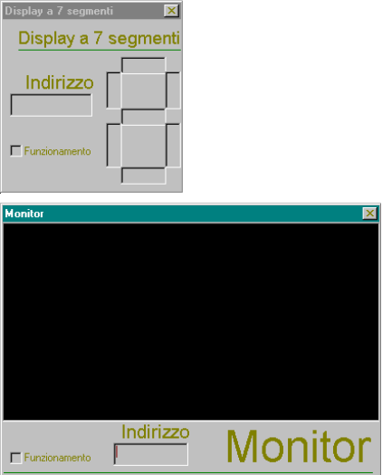
Usually, to send output data, an intermediate buffer is used in which the data are temporarily stored. In this simulator, however, the situation is slightly different. Here there is no intermediate buffer, and the data displayed directly on the monitor or on the 7-segment display are taken directly from the memory location whose address is clearly specified in the output forms.
This means that the output data are read directly from memory, without passing through an intermediate buffer, when they are ready to be displayed.
Conclusions
In conclusion, the simulator described offers a detailed approach to running and analysing programs written in assembly language. With a variety of features, including fast execution mode, debug mode and the graphical display of registers and memory, the simulator provides a versatile environment for analysing and testing programs.
Although some variations from reality were introduced to handle the input and output characteristics, these changes still make it possible to simulate the behaviour of a microprocessor effectively and to run assembly programs efficiently.
In addition, the ability to open files other than those created by the assembler gives greater flexibility in using the simulator.
Overall, this simulator is a valuable tool for students and computing enthusiasts who want to explore the world of assembly language and gain a thorough understanding of the internal workings of a microprocessor. The combination of graphical display, controlled execution and detailed program analysis makes it an important resource for learning and experimenting in computing.




I am the author of this page on “Assemblatore e Simulatore del Processore 6502 Realizzato in Visual Basic”. If something is unclear, if you need another example or want to go deeper into a point, write it in the comments below: I answer personally. If the page was useful, leave a star rating at the top of the article.