Markov decision processes: agent, environment, return, policy and value functions
The language of reinforcement learning: the agent-environment loop, the Markov property, return and discount, policy, state and action value, advantage, the gridworld with random and optimal policy.
https://www.electronics-engineering.com/en/markov-decision-processes-return-policy-value-functions/
In supervised learning someone provides the right answer for every example. In reinforcement learning (RL) nobody knows it: an agent tries actions in an environment, receives a numerical reward and must learn by itself which behaviour maximises it in the long run. This is how programs that play better than champions (AlphaGo), robots that walk, traffic controllers and the final stage of large language models (RLHF) are trained. This first lesson defines the mathematical language of the whole course: the Markov decision process, the return, the policy and the value functions.
The agent and the environment
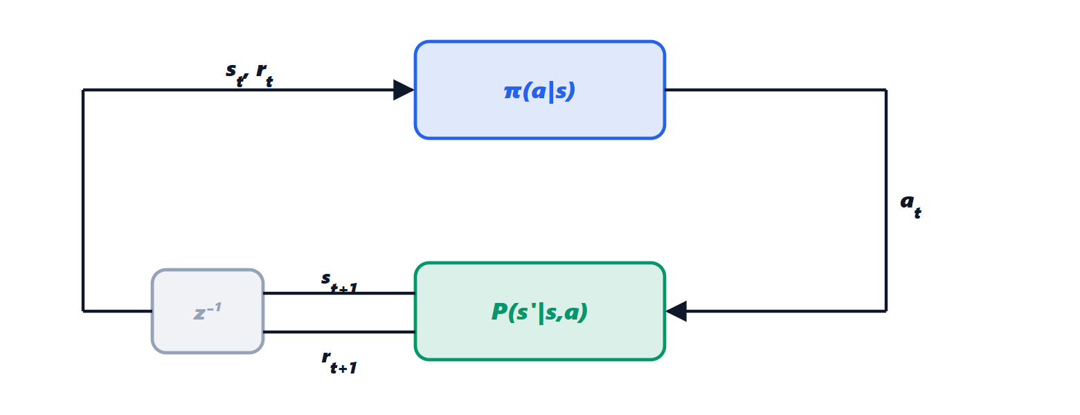
At each instant  the agent observes the state
 , chooses an action
 , and the environment responds with a reward
 and a new state
 . The loop repeats. For a robot the state is the joint positions and velocities, the action the motor torques, the reward a number that rewards moving forward without falling. For CartPole, the example we will use often, the state is the cart position and velocity, the pole angle and angular velocity, the action is pushing left or right, and the reward is +1 for every step in which the pole stays up.
The Markov decision process
An MDP (Markov decision process) is the five-tuple  :
 the set of states,
 that of actions;
 the probability of moving to
 by taking
 in
 ;
 the average reward obtained by taking in ;
 the discount factor.
The word Markov indicates the fundamental assumption: the future depends on the past only through the present state,  . If the observation does not contain everything needed (for example a single image of a ball, which does not tell its velocity), it is recovered by putting previous observations in the state too or by using networks with memory.
The return and discounting
The goal is not the immediate reward but the return, the sum of discounted future rewards:

Discounting has three reasons. Mathematical: if rewards are bounded by  and
 , the geometric series converges,
 . Practical: a distant reward is more uncertain. Interpretive:
 is the horizon over which the agent “looks”: with
 about 100 steps. The recursive relation, the basis of the whole course, holds:

Policy and value functions
A policy  is the rule by which the agent chooses: the probability of taking in state (deterministic if it always gives the same action). To evaluate it one defines:

 , the value of the state, is the average return starting from and following
 ;
 , the action value, is the average return taking first and then following . They are linked by
 . The difference
 is called the advantage: how much better than average action is. All modern algorithms use it.
A policy  is optimal if
 in every state, for every other . In a finite MDP a deterministic optimal policy always exists (this is proved in the lesson on Bellman equations), and knowing
 it is immediate:
 .
A complete example: the gridworld
A 4×4 grid; the top-left and bottom-right cells are the exits. The agent moves one cell up, down, left or right (if it hits the border it stays put), and each step costs  : maximising the return means leaving as soon as possible. With
 :
- for the optimal policy the value of each cell is minus the number of steps to the nearest exit: 0, −1, −2, −3;
- for the random policy (each direction with probability 1/4) the values are much more negative: −14 near the exits, −22 in the far corners, because the random walk wanders for a long time before leaving.
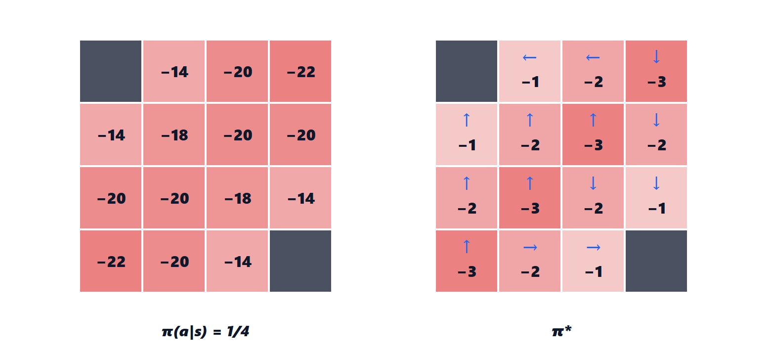
The fact that the random policy is worth −22 in a corner, and the optimal one −3, shows the central point of RL: from the same states and the same actions, the chosen behaviour changes the result radically. The next lesson shows how to compute these values, and from them the optimal policy, with the Bellman equations; the following lessons how to learn them when  and
 are unknown and the state is too large for a table.
Where RL sits among control techniques
Those who have studied Control Systems will recognise the structure: the state, the input (action), the dynamics (), a cost index to optimise ( ). Optimal control (LQR, MPC) solves the same problem knowing the model; RL solves it learning from experience, even when there is no model or it is too complicated. The price is the number of trials: this is why RL is almost always done in simulation, and the speed of simulators (lesson on libraries) is decisive.





Benvenuti nella pagina su «Processi decisionali di Markov: agente, ambiente, ritorno, policy e funzioni valore». L'ho scritta pensando a chi studia ingegneria elettronica: se un passaggio non vi torna, un esercizio vi dà un risultato diverso o volete altro materiale sull'argomento, chiedete pure nei commenti e vi risponderò. Un voto con le stelle qui sopra mi aiuta a capire quali pagine migliorare.Welcome to the page on “Markov decision processes: agent, environment, return, policy and value functions”. I wrote it for engineering students: if a step does not add up, an exercise gives you a different result or you would like more material on the topic, just ask in the comments and I will reply. A star rating above helps me understand which pages to improve.