Setting up controllers in multivariable systems: relay, Niederlinski, sequential method and BLT

In process plants (distillation columns, reactors, boilers) most systems have several inputs and several outputs, yet they are almost always controlled with separate PIDs, one per loop: this is decentralised control. It is simple, every operator understands what each controller does and, if one loop goes to manual, the others keep working. The price is that the loops disturb each other: a PID tuned well on its own can make the plant unstable when the other loops are closed too. This in-depth study shows how PIDs are set up (tuned) in this case: identification with the relay, checking interaction with the RGA and the Niederlinski index, the sequential method, the BLT method with the reasoning behind its criterion, and the detuning methods, all on the classic Wood and Berry column example, with Python code that reproduces the numbers. The linked lesson explains interaction, RGA and decoupling.

The subject was studied in the degree thesis of Eliana Li Santi at the University of Pisa (supervisors Aldo Balestrino and Alberto Landi, 2004), which compares the methods in simulation: the chapters are at the bottom of the page.

The example: the Wood and Berry column

It is the most used test process in the literature on multivariable control: a methanol-water distillation column in which the distillate purity and the bottoms purity are controlled by acting on the reflux flow and the reboiler steam . The identified model (times in minutes) is

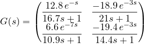
Each element is a first-order lag with dead time: each input acts on both outputs, with different delays.

Interaction. The relative gain of the pairing , is

Positive, so the pairing is the right one, but far from 1: closing loop 2 halves the gain that loop 1 sees (). A PID tuned on loop 1 alone will turn out about twice as aggressive as expected if the other loop is closed.

Niederlinski index. For a system with integral action in every loop,

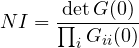
Theorem (Niederlinski). If , decentralised control with integral action cannot work safely with that pairing: either the system is unstable with all loops closed, or it becomes unstable when one of the loops is opened (put in manual, or saturated). The controllers have gains of the same sign as their , as always in practice.

Proof (slow controllers). Consider very slow pure integral controllers, with small : the most cautious tuning possible. The slow closed-loop poles are near the origin, where ; the characteristic equation becomes , with , so the slow poles are , with the eigenvalues of . The product of the eigenvalues is . Since has the sign of , has the sign of and so has the sign of . If the determinant is negative: a real matrix with negative determinant has an odd number of negative real eigenvalues, hence at least one and a pole . The system is unstable even with the slowest tuning. The general result, for any tuning, is due to Grosdidier, Morari and Holt (1985). ∎

For the column : the pairing is not excluded. For a 2×2 system always holds, and indeed here .

Identification with the relay

Tuning a PID with the Ziegler-Nichols rules needs the ultimate gain and the ultimate period . Bringing a plant to the stability limit by raising the gain is dangerous; Åström and Hägglund (1984) proposed replacing the controller with a relay: the controller output switches between and depending on the sign of the error. The loop settles into a stable oscillation of controlled amplitude ( is chosen), from which and are obtained. It is the basis of the autotuning function found in almost all industrial controllers.

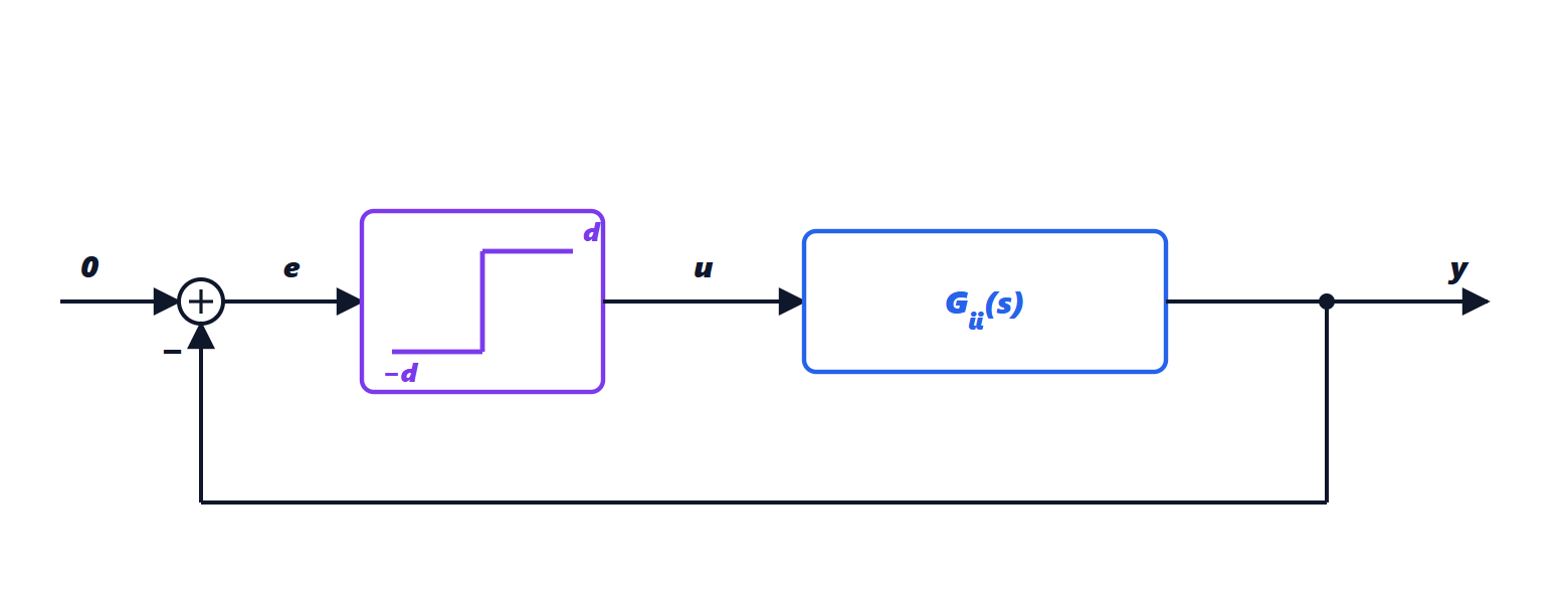
Theorem (relay describing function). If the output oscillates almost sinusoidally with amplitude , then

Proof. The relay output is a square wave of amplitude . Its Fourier series is . The process is a low-pass filter: higher harmonics are attenuated and only the first, of amplitude , matters. The relay therefore behaves as an equivalent gain (ratio between the first harmonic of the output and the input amplitude), in phase. An oscillation sustains itself when : the phase of must be ° and . But this is exactly the definition of the ultimate frequency and gain: . ∎

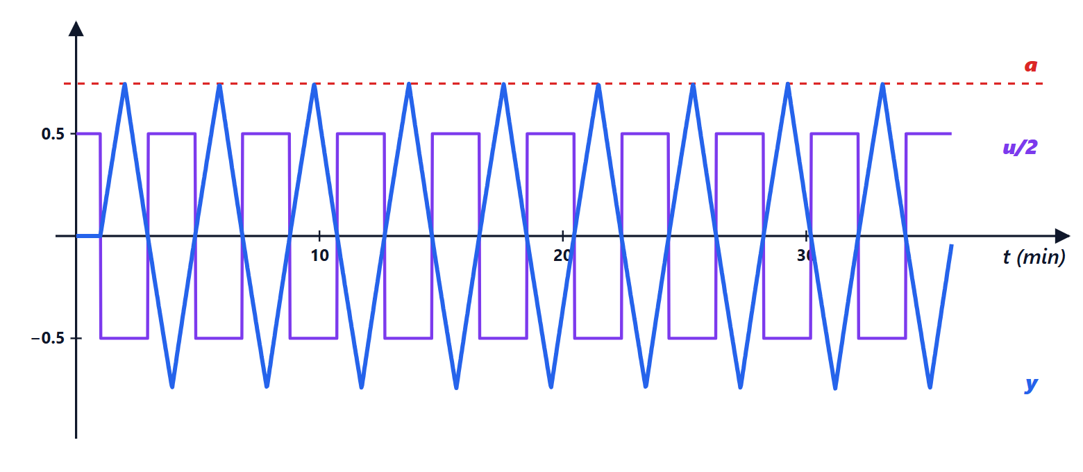
How accurate is it? Simulating the test on the two loops of the column (code below) and comparing with the exact calculation from the frequency response:

	exact	relay	exact	relay
loop 1	2.099	1.709	3.91 min	3.89 min
loop 2	0.422	0.349	11.13 min	10.97 min

The period is almost exact; the gain is underestimated by 17-19 %, because with a delay small compared with the time constant the output is more triangular than sinusoidal (as the graph shows) and the first-harmonic assumption is approximate. The error goes in the safe direction: a somewhat less aggressive controller results. Commercial controllers correct the estimate or add hysteresis to the relay to make it robust to noise.

Ziegler-Nichols loop by loop

With the exact and , the Ziegler-Nichols rules for the PI (, ) give

• loop 1: , min;
• loop 2: , min (negative because ).

Each one, on its own, works. But closing both loops makes the system unstable: in simulation the oscillation after the setpoint step does not die out and its amplitude slowly grows (0.248, 0.257, 0.266 in three successive 100-minute intervals). It is the consequence of : each loop sees a process different from the one it was tuned on.

The sequential method

The loops are tuned one at a time, closing them in order: first the fastest loop (here loop 1, min), with the relay test and the tuning rules; then, with loop 1 closed, the relay test is run on loop 2, which thus sees the “effective” process including the effect of the other loop. With more loops one continues, and the round can be repeated until the parameters stop changing. Advantage: each relay test accounts for the real interactions of the plant. Drawbacks: the result depends on the order, and the first loop, tuned while the others were open, may need retuning.

The BLT method

Luyben (1986) proposed a simple and widely used method, called BLT (biggest log-modulus tuning):

1. Compute the Ziegler-Nichols settings of each loop, and .

2. Choose a single detuning factor and set , : all loops become slower in the same proportion.

3. Compute the function

4. Choose so that the maximum of is dB, with the number of loops.

Why it works. By the multivariable Nyquist theorem, the closed-loop system is stable if the plot of does not encircle the origin (with process and controllers stable in open loop). is defined so that : the condition becomes “ does not encircle “, as in the Nyquist plot of a single loop with loop function . Then plays the role of the complementary sensitivity function, and its peak (the closed-loop resonance peak) measures how close the plot comes to . For a single loop the rule of thumb is a +2 dB peak; for loops Luyben uses dB because contains products of loop functions and grows faster. ∎

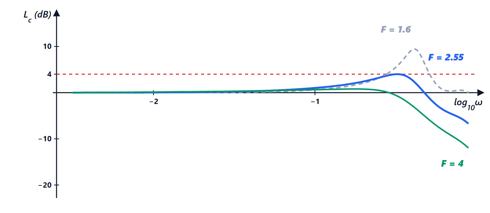
For the column, with a 4 dB peak is sought:

	1	2	2.5	3
peak of	50.1 dB	6.5 dB	4.2 dB	2.6 dB

With (uncorrected Ziegler-Nichols) the peak is very high: the plot passes almost through , consistent with the oscillation that does not decay. Solving for 4 dB gives (Luyben rounds it to 2.55), i.e.

• loop 1: , min;
• loop 2: , min,

the same values published by Luyben.

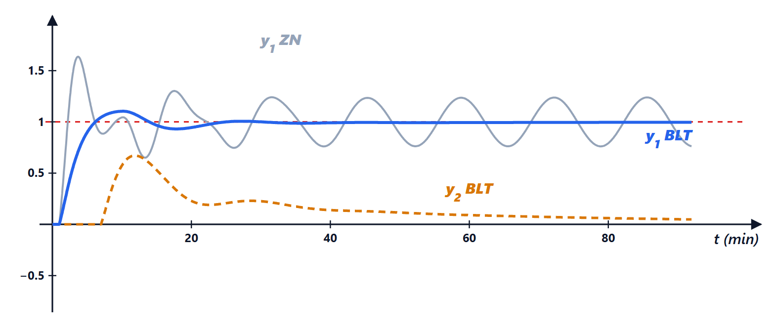
In the simulation of the setpoint step on , with the BLT settings has a 10 % overshoot and a maximum disturbance of 0.67; the integral of absolute error (IAE, summed over the two outputs in 120 minutes) is 19.7, against 76.3 for Ziegler-Nichols, which would however keep growing because the system is unstable.

Other detuning methods

BLT’s single factor is safe but not optimal: it also slows down the loop that would not need it. Later methods, also compared in the thesis, seek better compromises:

• detuning with integral criteria: is chosen by minimising an index such as IAE or ISE computed in simulation on the complete system, instead of with the peak of ;
• detuning with different factors: one factor per loop, , chosen with the same criterion; the more coupled loops are slowed down more;
• iterative detuning: start from and increase it in steps on the real plant until the response is acceptable; it needs no model, only tests;
• conditional integration: this is anti-windup. When a controller output saturates (a valve fully open), the integral stops accumulating; without this precaution, in multivariable systems a saturated loop drags the others into long oscillations.

In industrial practice the typical sequence is: RGA and Niederlinski to choose the pairings, relay test for each loop, BLT for a safe starting tuning, fine-tuning on the plant. If interaction is too strong ( very different from 1) one moves to decouplers or predictive control (MPC), described in the lesson.

The Python code

The program computes RGA and Niederlinski, the exact ultimate gain and period, simulates the relay test and finds the BLT factor:

import numpy as np
from scipy.optimize import brentq

# Wood-Berry column: G_ij = K e^{-theta s} / (tau s + 1), times in minutes
K = np.array([[12.8, -18.9], [6.6, -19.4]])
TAU = np.array([[16.7, 21.0], [10.9, 14.4]])
TH = np.array([[1.0, 3.0], [7.0, 3.0]])

def G(s):
    return K * np.exp(-TH * s) / (TAU * s + 1)

l11 = 1 / (1 - K[0, 1] * K[1, 0] / (K[0, 0] * K[1, 1]))
NI = np.linalg.det(K) / (K[0, 0] * K[1, 1])
print(f"RGA lambda11 = {l11:.3f}, Niederlinski = {NI:.3f}")

# exact ultimate gain and period (phase = -180 degrees) and Ziegler-Nichols rules for the PI
ZN = []
for i in range(2):
    phase = lambda w: -TH[i, i] * w - np.arctan(TAU[i, i] * w) + np.pi
    wu = brentq(phase, 1e-3, 10)
    Ku = np.sqrt(1 + (TAU[i, i] * wu) ** 2) / abs(K[i, i])
    Pu = 2 * np.pi / wu
    ZN.append((np.sign(K[i, i]) * Ku / 2.2, Pu / 1.2))
    print(f"loop {i+1}: Ku = {Ku:.3f}, Pu = {Pu:.2f} min, PI: Kc = {ZN[i][0]:.3f}, TI = {ZN[i][1]:.2f}")

# simulated relay test (d = 1, Euler with 2 ms step, delay as a sample queue)
def relay(i, d=1.0, dt=0.002, T=150):
    n, nd = int(T / dt), int(round(TH[i, i] / dt))
    u_queue, y, ys = np.zeros(n + nd), 0.0, np.zeros(n)
    for k in range(n):
        u_queue[k + nd] = -d * np.sign(K[i, i]) if y > 0 else d * np.sign(K[i, i])
        y += dt * (-y + K[i, i] * u_queue[k]) / TAU[i, i]
        ys[k] = y
    tail = ys[n // 2:]
    a = (tail.max() - tail.min()) / 2
    rises = np.where(np.diff(np.sign(tail)) > 0)[0]
    return 4 * d / (np.pi * a), np.mean(np.diff(rises)) * dt

for i in range(2):
    Ku_r, Pu_r = relay(i)
    print(f"relay loop {i+1}: Ku = {Ku_r:.3f}, Pu = {Pu_r:.2f} min")

# BLT: peak of Luyben's log modulus equal to 2N = 4 dB
def peak_Lc(F):
    peak = -np.inf
    for w in np.logspace(-3, 1, 4000):
        s = 1j * w
        Gc = np.diag([ZN[j][0] / F * (1 + 1 / (F * ZN[j][1] * s)) for j in range(2)])
        W = -1 + np.linalg.det(np.eye(2) + G(s) @ Gc)
        peak = max(peak, 20 * np.log10(abs(W / (1 + W))))
    return peak

F = brentq(lambda F: peak_Lc(F) - 4.0, 1.2, 5)
print(f"BLT: F = {F:.3f}")
for j in range(2):
    print(f"loop {j+1}: Kc = {ZN[j][0] / F:.3f}, TI = {ZN[j][1] * F:.2f} min")

Running it prints , , the ultimate and Ziegler-Nichols values of the table, and the BLT settings. In MATLAB the same calculation is done with tf with the InputDelay property, allmargin for the ultimate values and freqresp for .

The original thesis

The chapters of the thesis by Eliana Li Santi, *Predisposizione dei controllori nei sistemi multivariabili* (Setting up controllers in multivariable systems), University of Pisa, 2004, in Italian, with implementations and comparisons in simulation:

• Title page and contents
• Chapter 1: PID model, relay identification
• Chapter 2: sequential method
• Chapter 3: BLT
• Chapter 4: detuning with integral criteria, noise robustness, multivariable Nyquist
• Chapter 5: detuning with conditional integration, saturation
• Chapter 6: detuning with different factors
• Chapter 7: iterative detuning
• Conclusions and bibliography