Antenna radiation pattern: lobes, beamwidth and directivity
How to read an antenna radiation pattern: main and side lobes, half-power beamwidth, directivity, gain, front-to-back ratio, with a MATLAB script.
https://www.electronics-engineering.com/articolo_169-diagramma_di_irradiazione_tridimensionale.htm
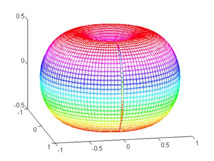
The radiation pattern of an antenna tells you how the radiated power is distributed in space: in which directions the antenna sends (or receives) most of its energy, and where it is almost deaf. It is a three-dimensional shape, but in practice we almost always look at two cuts through it: a horizontal one and a vertical one.
Being able to read a pattern is essential when choosing an antenna for a radio link, a radar or a Wi-Fi access point, so here are the quantities you will find on any datasheet and how they are defined.
Lobes
A directional antenna concentrates power in one region, the main lobe (or main beam). Around it there are smaller peaks, the side lobes, and often one pointing the opposite way, the back lobe. Side lobes are unwanted: they waste power, pick up interference from directions you are not interested in and, in a radar or IFF system, can produce false echoes. The side lobe level (how many dB the strongest side lobe is below the main beam) is therefore one of the first figures to check.
The figure below is a two-dimensional pattern of this kind: main lobe in red, back lobe on the opposite side and side lobes in grey.
Beamwidth
- Half-power beamwidth (HPBW): the angle between the two directions where the radiated power drops to half of the maximum, i.e. −3 dB. This is the number usually quoted as “beamwidth”.
- First-null beamwidth (FNBW): the angle between the first two nulls on either side of the main lobe. It is always larger than the HPBW.
Narrow beams give better angular resolution and more range, but the antenna has to be pointed more accurately.
Directivity, gain and front-to-back ratio
Directivity compares the radiation intensity in the strongest direction with that of an ideal isotropic antenna radiating the same total power equally in all directions. Gain is the directivity multiplied by the antenna efficiency, so it also accounts for losses in conductors and dielectrics. Both are given in dBi (decibels relative to isotropic); sometimes you will find dBd, relative to a half-wave dipole, and the two differ by 2.15 dB.
The front-to-back ratio is the difference in dB between the main lobe and the back lobe. It matters a lot for point-to-point links and for TV antennas, where you want to reject signals arriving from behind.
How patterns are plotted
Patterns are drawn either in polar form, which gives an immediate picture of the shape, or in rectangular form (angle on the horizontal axis, level on the vertical one), which makes it easier to read beamwidths and side lobe levels. In both cases the values are normally normalised to the maximum and expressed in dB, so the peak of the main lobe is at 0 dB.
Two classic examples
The short dipole (Hertzian dipole, a current element much shorter than the wavelength) has a field proportional to sin θ, where θ is measured from the dipole axis. In the plane containing the dipole the pattern is a figure of eight with nulls along the axis; in the perpendicular plane it is a circle, so the antenna is omnidirectional around its axis. Its directivity is 1.5 (1.76 dBi) and its half-power beamwidth is 90°, because sin²θ falls to one half at θ = 45° and θ = 135°.
The half-wave dipole has a slightly narrower doughnut: directivity 1.64 (2.15 dBi) and a beamwidth of about 78°. Adding elements, as in a Yagi-Uda array or a patch array, squeezes the doughnut into a single main beam with higher gain and visible side lobes.
Plotting the 3D pattern of a current element in MATLAB
The short script below draws the three-dimensional pattern of a short dipole, |E| ∝ sin θ, by converting the spherical surface to Cartesian coordinates. Changing the line that defines E lets you plot other patterns, for example abs(cos(pi/2*cos(TH))./sin(TH)) for the half-wave dipole.
% 3D radiation pattern of a short current element (|E| proportional to sin(theta))
clear; clc;
theta = linspace(0, pi, 91);          % angle from the dipole axis
phi   = linspace(0, 2*pi, 181);       % azimuth
[TH, PH] = meshgrid(theta, phi);

E = abs(sin(TH));                     % normalised field pattern

% spherical to Cartesian (sph2cart wants elevation, i.e. pi/2 - theta)
[x, y, z] = sph2cart(PH, pi/2 - TH, E);

surf(x, y, z, E, 'EdgeColor', 'none');
axis equal; colorbar; grid on;
xlabel('x'); ylabel('y'); zlabel('z (dipole axis)');
title('Short dipole: 3D radiation pattern');
view(30, 20);


Welcome to the page on “Antenna radiation pattern: lobes, beamwidth and directivity”. I wrote it for engineering students: if a step does not add up, an exercise gives you a different result or you would like more material on the topic, just ask in the comments and I will reply. A star rating above helps me understand which pages to improve.