Limit of a composite function: theorem, proof and change of variable
When you can move a limit inside a function: statement, epsilon-delta proof, a counterexample, change of variable and worked examples.
When you compute a limit such as  it feels natural to “move the limit inside”: first find the limit of
 , which is 1, then take the square root. You do this dozens of times in every exercise, but it is not always allowed. The theorem on the limit of a composite function says exactly when it is.
The statement
Let  be defined in a neighbourhood of
 (except possibly at ) and
 defined in a neighbourhood of
 . If
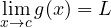 , and
- is continuous at ,
then

In words: a continuous function “commutes” with the limit.
The epsilon-delta proof
Fix  . We need a
 such that
 implies
 . We build it in two steps, starting from the end.
- Continuity of at . There is
 such that
 . So it is enough for
 to land within
 of .
- Limit of . Apply the definition of limit with in place of epsilon: there is such that
 .
Putting the two together: if , then  , and therefore . Since
 was arbitrary, the limit is
 . ∎
The key point is that the  for is chosen after receiving the from : the two definitions mesh like two gears.
Why continuity is needed: a counterexample
If only has a limit at , without being continuous there, the result can fail. Take

We have  and
 . But
 for every
 , so
 , not 0. The trouble is that “lands” exactly on the point where jumps.
There is also a version of the theorem without continuity: if  and
 in a neighbourhood of (except at ), then
 . This is what justifies a change of variable in limits.
How it is used in exercises
Example 1.  . The exponent tends to 1 (a standard limit) and the exponential is continuous, so the limit is
 .
Example 2 (change of variable). 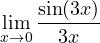 . Set
 : as
 , also
 , and
 when
 . The limit becomes
 .
Example 3. 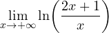 . The argument tends to 2, the logarithm is continuous at 2, so the limit is
 .
Almost every function you meet (polynomials, exponentials, logarithms, sine and cosine, roots) is continuous on its domain, which is why “moving the limit inside” works so often. Mistakes happen when the argument tends to a point outside the domain (the logarithm of something that tends to 0) or to a point of discontinuity, such as the integer part of a number that tends to an integer.
The same theorem with sequences
Continuity can also be characterised with sequences: is continuous at if and only if  for every sequence
 . This gives the same result: if
 and is continuous at , then
 . That is why, for instance,
 .

