Fixed and variable costs, break-even and operating leverage
Contribution margin, the break-even point proved with an example, margin of safety, the degree of operating leverage proved, the effect of discounts, limits of the linear model.
How many units must be sold to avoid a loss? How much does profit grow if sales rise by 10 %? Is it worth lowering the price to sell more? The answers come from the distinction between fixed and variable costs. In this lesson we look at cost behaviour, the break-even point with its proof and an example, the margin of safety, operating leverage with its proof, and the limits of the model.
Fixed and variable costs
With respect to the production volume  , within a reasonable range:
- fixed costs
 do not change: rents, salaries of overhead staff, depreciation of plant, insurance;
- variable costs grow proportionally: raw materials, components, process energy, commissions. With unit variable cost
 , they amount to
 .
Total cost is  , revenues
 with unit price
 . The difference
 is the unit contribution margin: what each unit sold brings to cover fixed costs and then profit.
The break-even point
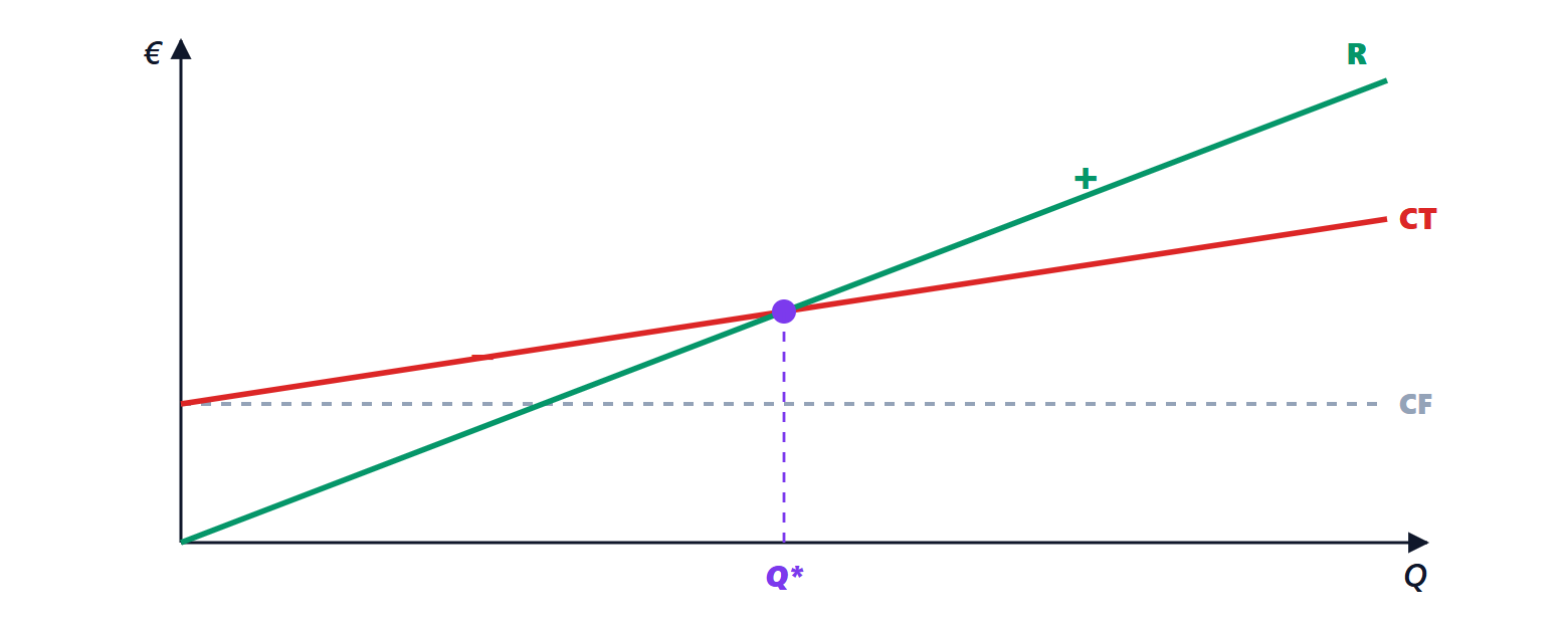
Theorem. The volume at which the operating result is zero is
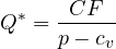
and the corresponding turnover is  .
Proof. The operating result is  , linear in and increasing if
 . It vanishes for
 . Multiplying by :
 . ∎
The break-even point is therefore the number of “contribution margins” needed to pay the fixed costs.
Example. A company makes a device sold at 2.5 (hundreds of euros) with variable costs of 1.0 and annual fixed costs of 60,000 (hundreds of euros):  units. If it sells 60,000, the operating result is
 .
The margin of safety  measures how far sales can fall before a loss: here
 %.
Operating leverage
A company with many fixed costs and few variable ones (a semiconductor fab, an airline, a software company) has results very sensitive to volume; one with many variable costs (a trading company) less so.
Theorem. The degree of operating leverage

is the ratio between the percentage change in operating result and that in volume.
Proof. If volume changes by  , the operating result changes by
 , because fixed costs do not change. The relative change is

and the factor in front of  is the total contribution margin
 divided by
 . ∎
Example. With the previous numbers, at 60,000 units  and
 :
 . A 10 % increase in sales (66,000 units) raises the operating result by 30 %, to 39,000; a 10 % drop lowers it by 30 %. Near the break-even point leverage becomes enormous, because in the denominator tends to zero. It is the operating analogue of financial leverage (lesson on ratios), and the two multiply.
Pricing decisions
The model helps evaluate a price cut: if the price falls from to  , keeping the same result requires sales
 . With a 10 % discount in the example (
 ), the unit margin falls from 1.5 to 1.25 and 20 % more units are needed just to stay even: discounts cost more than they seem when the contribution margin is small.
Limits of the model
Linearity holds only within a relevant range: beyond a certain output a second shift or a new plant is needed, and fixed costs rise in steps; unit variable costs may fall with volume discounts or rise with overtime; the price may have to fall to sell more. With several products the break-even point depends on the sales mix. The chart nevertheless remains a quick and very powerful tool for reasoning about prices, volumes and cost structure, and for comparing technologies with different fixed and variable costs (lesson on cost accounting).