Budget, cash and variance analysis
The budget cascade, the cash conversion cycle proved with an example, working capital needs during growth, the price and volume variance decomposition proved.
Companies do not fail for lack of profit, but for lack of cash: a growing company, with good orders and margins, can find itself without money to pay wages and suppliers, because it has paid in advance for materials and labour and the customers have not yet paid. In this lesson we look at the budget, the cash conversion cycle with its proof and an example, the working capital requirement, and variance analysis with its proven decomposition into price effect and volume effect.
The budget
The budget translates the year’s goals into numbers, and is used to coordinate departments and monitor progress. It is built as a cascade:
- sales budget: quantities and prices per product and market, the starting point and the most uncertain estimate;
- production budget: quantities to produce, taking desired inventories into account;
- budgets for materials, labour, overheads, investments;
- forecast income statement and balance sheet;
- cash budget: receipts and payments month by month, telling whether and when financing will be needed.
During the year actual values are compared with forecast ones (management control), and action is taken on significant variances.
The working capital cycle
Time passes between paying suppliers and collecting from customers, and that time must be financed.
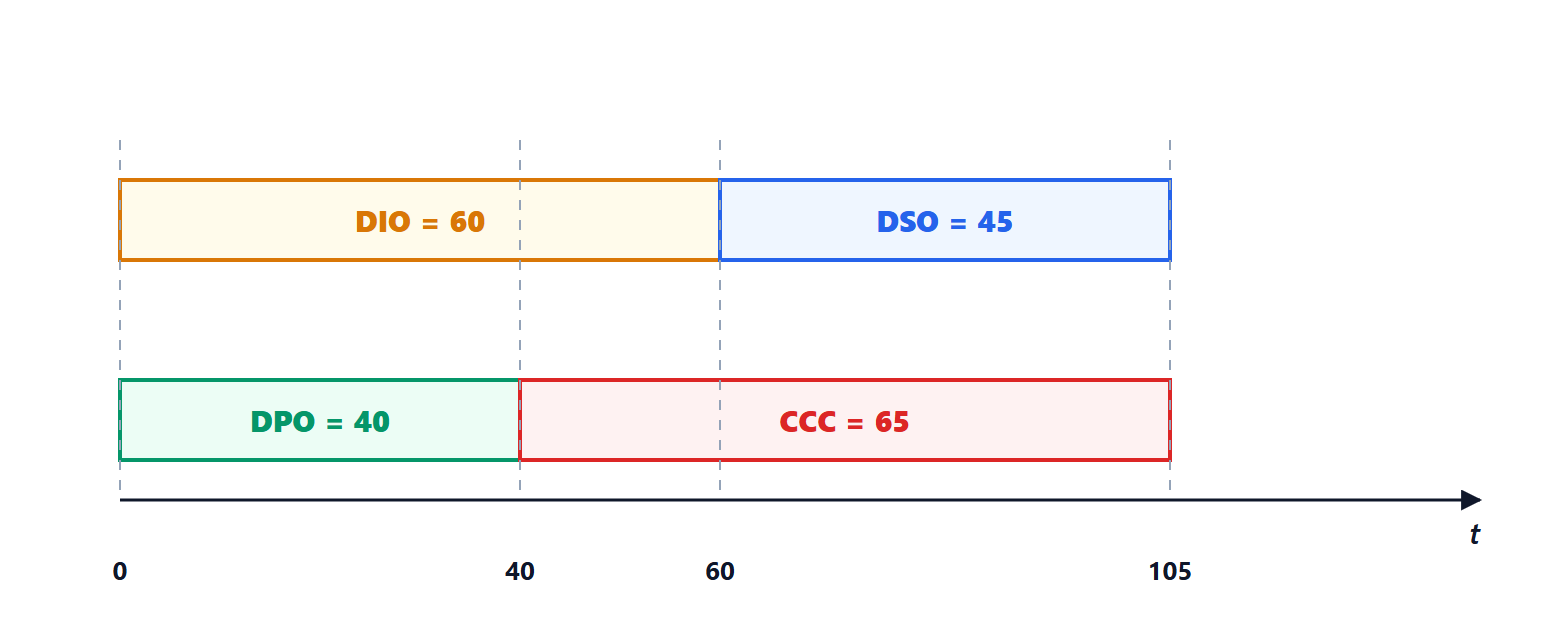
The average days of inventory (DIO), of collection from customers (DSO) and of payment to suppliers (DPO) are defined, for example  .
Theorem. The average time between paying suppliers and collecting from customers, the cash conversion cycle, is

Proof. Follow a unit of material along the time line, starting from its arrival in the company (day 0). It stays in inventory, as material and then as product, until it is sold, on average on day  ; the customer pays on average on day
 . The supplier was paid on day
 . The interval in which the company has already paid but not yet collected runs from to , and lasts
 . ∎
Example. With 60, 45 and 40 days,  days. With a turnover of 3.65 million euros a year, i.e. 10,000 euros a day, the company must permanently finance about 65 days of activity: of the order of 650,000 euros (valuing everything at selling price; at cost the requirement is somewhat lower). Reducing collection time by 15 days frees about 150,000 euros of cash, without selling a single extra unit.
Growth costs cash
The working capital requirement is proportional to turnover: if sales grow by 30 %, the capital to be financed also grows by 30 %. A fast-growing company absorbs cash even if it is very profitable, and must plan short-term financing in good time (lesson on financing). The levers for shortening the cycle are inventory (lean production, frequent deliveries, Business Management and Logistics lessons), collection times (prompt invoicing, reminders, factoring) and payment times, consistent with supplier relationships.
Variance analysis
If actual revenues differ from forecast ones, one must understand why: was more or less sold, or at different prices?
Theorem. The difference between actual revenues  and forecast revenues
 decomposes exactly into

Proof. Add and subtract  :
 , and factor. ∎
Example. Forecast 1000 units at 50 euros (50,000), actual 1100 at 48 (52,800). Price variance  , volume variance
 : total
 . Sales went better than forecast in quantity, but with discounts that ate up a third of the gain: these are different pieces of information, for different managers. The same decomposition applies to costs (purchase price variances, efficiency in the use of materials and labour) and makes it possible to attribute each difference to whoever controls it.