The intermediate zero theorem (Bolzano): statement and proof by bisection
A continuous function that changes sign on a closed interval has a zero: proof by bisection, a numerical example, applications and what the theorem does not say.
The intermediate zero theorem (also called Bolzano’s theorem) looks obvious at first sight: if a continuous function starts below the x axis and ends above it, it has to cross it somewhere. Proving it properly, though, requires a property of the real numbers that is usually taken for granted, completeness. That is exactly why the proof is worth studying.
The statement
Let  be a continuous function on the closed and bounded interval
 , and suppose that
 and
 have opposite signs, that is
 . Then there is at least one point
 such that

Every hypothesis matters. If the interval is not closed, or if the function has even a single jump, the zero can be missing: the function equal to  for
 and to
 for
 changes sign on
 but never vanishes.
Do not go round in circles
You will often see this theorem “proved” by quoting the intermediate value theorem. The argument is not wrong in itself, but in most first-year calculus courses the order is the other way round: the zero theorem comes first, and the intermediate value theorem is derived from it by applying it to  . Using the second to prove the first means assuming what you want to show. The classic proof, which we follow here, uses bisection.
The proof by bisection
Without loss of generality assume  (in the opposite case work with
 ). Set
 ,
 and build a sequence of smaller and smaller intervals.
- Take the midpoint
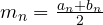 .
- If
 we have found the zero and we stop.
- If
 set
 ,
 ; if instead
 set
 ,
 .
If the procedure never stops, we get intervals  with three properties:
 (the left ends never decrease) and
 (the right ends never increase);
- the length halves at every step:
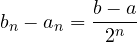 ;
- at every step
 still holds, because we always keep the half where the sign changes.
The sequence  is increasing and bounded above by
 . This is where completeness comes in: in the real numbers a monotone bounded sequence has a limit. Call
 the limit of . Since
 ,
 tends to as well, and clearly
 .
Now use the continuity of at :

The first inequality holds because all the values  are negative, and the limit of negative numbers is less than or equal to zero (sign is only preserved in the weak sense); the second comes in the same way from the positive values
 . The only number that is both
 and
 is zero, so
 . Finally cannot be
 or , because does not vanish there: hence . ∎
A worked example
Take  on
 :
 ,
 . The theorem guarantees a zero, which we know to be
 . Here are the first bisection steps:
| n | an | bn | mn | f(mn) |
|---|---|---|---|---|
| 0 | 1 | 2 | 1.5 | +1.375 |
| 1 | 1 | 1.5 | 1.25 | −0.047 |
| 2 | 1.25 | 1.5 | 1.375 | +0.600 |
| 3 | 1.25 | 1.375 | 1.3125 | +0.261 |
| 4 | 1.25 | 1.3125 | 1.28125 | +0.103 |
After  steps the error is at most
 : about ten iterations give three correct decimals. This is exactly the bisection method taught in numerical analysis: the proof of the theorem is also an algorithm, slow but impossible to break.
Where it is used
- Existence of solutions. The equation
 has a solution in
 : apply the theorem to
 , which is
 at 0 and
 at 1.
- Odd-degree polynomials. Every polynomial of odd degree has at least one real root, because as
 it takes values of opposite sign.
- Intermediate value theorem. If is continuous on , it takes every value between and : apply the zero theorem to .
- Electronics. Finding the operating point of a non-linear circuit (a diode in series with a resistor, for example) leads to an equation
 . Knowing that a solution exists in a given interval is the first step before looking for it with a numerical method.
What the theorem does not say
It guarantees at least one zero, not exactly one:  on
 changes sign between the endpoints and has four zeros. Uniqueness needs extra information, for instance that is strictly monotone. And the converse is false: a function can vanish without changing sign, like
 at 0, and there the theorem is of no help.




