The discrete Fourier transform (DFT): from the DTFT, inverse, properties and circular convolution proved

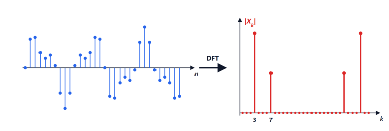
The discrete Fourier transform (DFT) is the transform a computer can actually compute: it takes numbers and returns numbers. Every digital spectrum analyser, every equaliser, every OFDM modem (Wi-Fi, 4G, 5G) and every fast filter uses it, almost always through the FFT algorithm. This in-depth study derives the DFT from the discrete-time Fourier transform (DTFT) and proves its formulas and properties: inverse transform, Parseval, circular shift, Hermitian symmetry, circular convolution and how to obtain linear convolution from it. The linked lessons explain the FFT algorithm and practical use in spectral analysis (leakage, windows, Welch’s method). The path follows the topics of Sandro Petrizzelli’s notes from which this page originated.

From the DTFT to the DFT

A sequence has DTFT

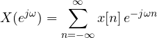
a continuous function, periodic with period in the normalised angular frequency . A computer cannot store a continuous function: it takes equally spaced samples of it, , . If is nonzero only for , these samples are

This is the -point DFT. The number is an -th root of unity: , and its powers are equally spaced points on the unit circle.

Theorem (sampling in frequency is repeating in time). If is longer than , the samples of its DTFT coincide with the DFT of the sequence , : the parts of beyond overlap (time aliasing).

Proof. Split the DTFT sum into blocks of samples, with : . Since , what remains is , the DFT of . ∎

It is the dual of the sampling theorem: sampling in time makes the spectrum periodic, sampling the spectrum makes the signal periodic. This is why the DFT always treats the block of samples as if it were one period of a periodic signal: all the properties that follow are “circular”.

The inverse transform

Theorem. .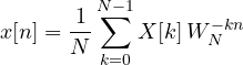

Proof. A lemma is needed, the orthogonality of discrete exponentials: if is a multiple of , otherwise 0. Indeed in the first case every term equals 1; in the second and the geometric sum is 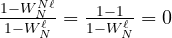. Now substitute the definition:

The inner sum equals only for (with between 0 and , is a multiple of only if it is zero): remains. ∎

In matrix form with , and the theorem says 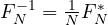: the matrix is unitary. Parseval’s theorem follows immediately:

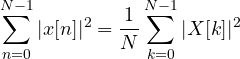
because a unitary matrix preserves the norm: 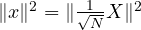. Energy can be measured equally in time or in frequency.

The properties, proved

In all that follows indices are taken modulo : is the remainder of divided by .

Linearity. : the definition is a sum.

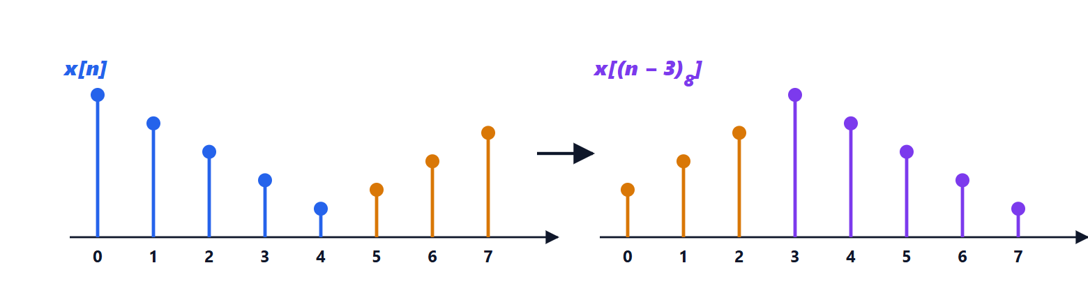
Circular time shift. .

Proof. ; with , as runs over so does (in another order), and because . The sum becomes . ∎

The delay only changes the phase of the coefficients, not the magnitude. But it is a circular delay: samples leaving on the right re-enter on the left.

Frequency shift (modulation). : same proof with the roles swapped. Multiplying by a complex exponential shifts the spectrum: it is the principle of frequency conversion in digital receivers.

Hermitian symmetry. If is real, .

Proof. , because . For real , conjugation only changes the sign of the exponent: . ∎

So real part and magnitude are symmetric about , imaginary part and phase antisymmetric: for a real signal the coefficients from 0 to are enough, and the “real” FFT does half the computation. The coefficient (with even ) is the Nyquist frequency and is real.

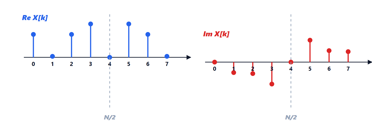
Circular symmetry. If moreover (even in the circular sense, i.e. ), the DFT is real; if it is odd, purely imaginary. It follows from the previous property: for even , .

Circular convolution

Theorem. The product of DFTs corresponds to circular convolution:

Proof. Compute the DFT of and use the circular shift: . ∎

Filtering a signal is instead a linear convolution, , with length if and have lengths and . Circular convolution on points is the linear one “wrapped around”: samples beyond are added at the start (the frequency-sampling theorem applied to ).

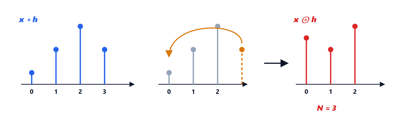
Example. , . The linear convolution is . With an point DFT the last 3 wraps onto : , a wrong result for a filter. With there is no overlap and is obtained again.

Practical rule: to filter with the FFT, pad and with zeros up to . For long signals the signal is split into blocks and the overlap-add and overlap-save methods are used, which reassemble the blocks without errors; with large the cost, instead of , is much lower than direct convolution.

Two DFTs to know by heart

Rectangular pulse of samples on points: with the geometric sum

(factoring in the numerator and in the denominator). The magnitude is the Dirichlet kernel, the discrete version of the sinc: for , it is . It is also the response of the rectangular window, the origin of spectral leakage.

Cosine on a bin. : by orthogonality the DFT equals at and at , zero elsewhere. If the frequency does not fall exactly on a bin the DFT has values at all : this is spectral leakage, covered in the spectral analysis lesson.

Zero padding

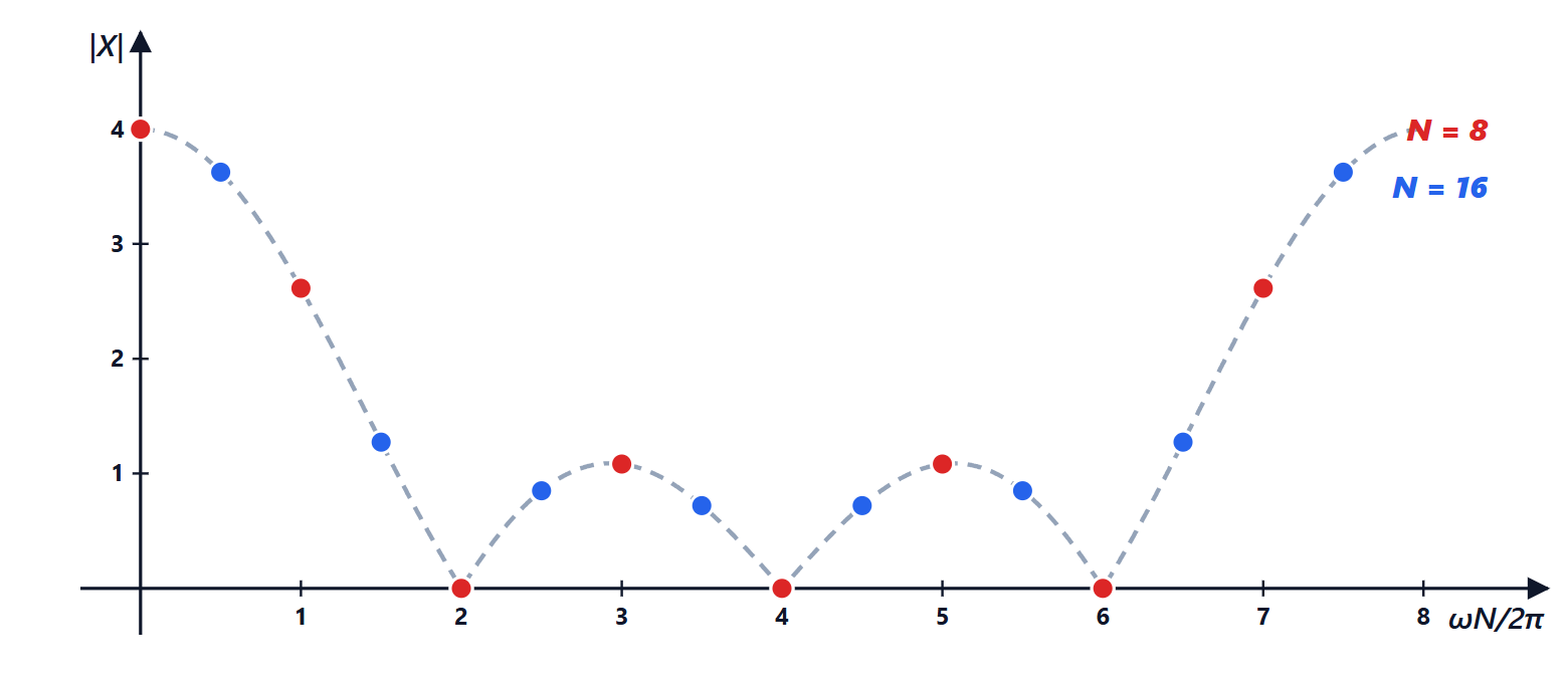
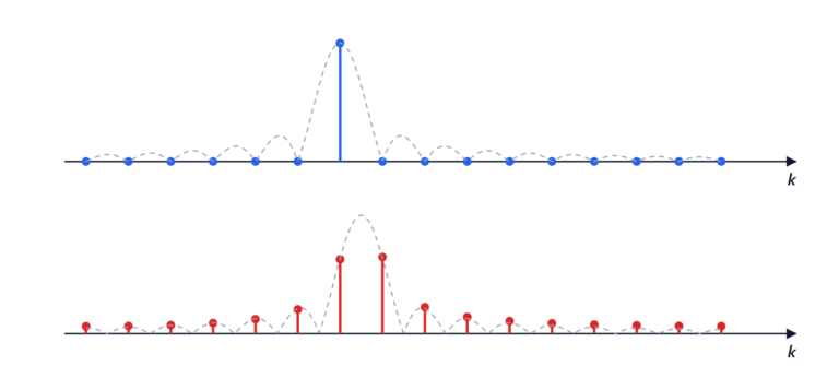
Padding a block of samples with zeros up to does not add information: by the first theorem, the -point DFT samples the same DTFT more densely (figure at the top, 8 and 16 points). It helps to read peak positions better and to reach a power of 2 for the FFT, but the ability to separate two close frequencies depends only on the duration of the observed signal: about .

Checking in Python

import numpy as np

def dft(x):
    """DFT from the definition: X[k] = sum x[n] e^{-j 2 pi k n / N}."""
    N = len(x)
    n = np.arange(N)
    W = np.exp(-2j * np.pi * np.outer(n, n) / N)     # Fourier matrix
    return W @ x

def idft(X):
    N = len(X)
    n = np.arange(N)
    return np.exp(2j * np.pi * np.outer(n, n) / N) @ X / N

rng = np.random.default_rng(1)
x = rng.standard_normal(8)
X = dft(x)
print("equal to np.fft.fft:", np.allclose(X, np.fft.fft(x)))
print("exact inverse:", np.allclose(idft(X), x))
print("Parseval:", np.isclose(np.sum(x**2), np.sum(abs(X)**2) / 8))
print("Hermitian symmetry X[N-k] = X*[k]:", np.allclose(X[1:][::-1], np.conj(X[1:])))
m = 3
print("circular shift:", np.allclose(dft(np.roll(x, m)), np.exp(-2j * np.pi * np.arange(8) * m / 8) * X))

# circular versus linear convolution
a, h = np.array([1.0, 2, 3]), np.array([1.0, 1])
lin = np.convolve(a, h)
circ3 = np.real(idft(dft(a) * dft(np.r_[h, 0])))
circ4 = np.real(idft(dft(np.r_[a, 0]) * dft(np.r_[h, 0, 0])))
print("linear:", lin, " circular N=3:", np.round(circ3, 6), " circular N=4:", np.round(circ4, 6))

# DFT of a rectangular pulse of L = 4 samples on N = 8 points: Dirichlet kernel
L, N = 4, 8
r = np.r_[np.ones(L), np.zeros(N - L)]
k = np.arange(1, N)
dirichlet = np.exp(-1j * np.pi * k * (L - 1) / N) * np.sin(np.pi * k * L / N) / np.sin(np.pi * k / N)
print("rectangle, Dirichlet formula:", np.allclose(dft(r)[1:], dirichlet), " |X| =", np.round(abs(dft(r)), 3))

# cosine falling exactly on bin 2
c = np.cos(2 * np.pi * 2 * np.arange(N) / N)
print("cosine on bin 2:", np.round(abs(dft(c)), 6))

All checks print True; the 3-point circular convolution gives and the 4-point one , equal to the linear one; the magnitude of the rectangle and the cosine on bin 2 (value 4 at and ) match the formulas. The DFT from the definition costs multiplications: for it does not matter, for it does, and this is the reason for the FFT algorithm, explained in the linked lesson.