Finite differences for hyperbolic equations: upwind, Lax-Wendroff and the CFL condition
The advection equation, instability of the centred scheme by von Neumann analysis, upwind and numerical diffusion, Lax-Friedrichs, Lax-Wendroff, Godunov's theorem and transmission lines.
This in-depth page completes the lesson on finite differences with the class of equations that is hardest to solve numerically: hyperbolic equations, which describe transport and propagation at finite speed, such as a pollutant carried by a river, a signal on a transmission line, a shock wave. We start from the simplest model, the linear advection equation, and see why the most “natural” scheme is unstable, how it is fixed and what the Courant condition says.
The advection equation

has the exact solution  : the initial profile moves right at speed
 without changing shape. Along the characteristics
 the solution is constant: information travels from left to right. It is an ideal test case, because the exact solution is known and any distortion of the profile is an error of the method.
The centred scheme is unstable
With a forward difference in time and a centred one in space, the most accurate:

It looks reasonable, but it is unstable for every  . To see this, use von Neumann analysis: substitute
 (a wave of wavenumber
 ) and compute the amplification factor
 :

Every component grows at every step. The scheme is consistent but not stable, and by the Lax-Richtmyer theorem it does not converge.
The upwind scheme
The fix is to look where the information comes from. With  it comes from the left, so use the backward difference:

If  the new value is a weighted average with positive weights: the scheme is stable and creates no oscillations. The amplification factor has
 exactly when
 : the Courant-Friedrichs-Lewy condition. With
 the scheme is exact (
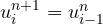 , the profile moves one cell per step).
The price is accuracy: upwind is first order and introduces numerical diffusion. A step is carried along but its corners are gradually rounded, as if there were a small diffusion term the true equation does not have. Writing the modified equation shows it: the scheme actually solves  .
Lax-Friedrichs and Lax-Wendroff
- Lax-Friedrichs replaces
 in the centred scheme with the average of the neighbours,
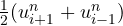 . It becomes stable for , but it is even more diffusive than upwind.
- Lax-Wendroff uses the second-order Taylor expansion in time and the equation itself to substitute
 :

It is second order and stable for , with little diffusion. But near jumps it produces spurious oscillations (overshoots before and after the step), similar to the Gibbs phenomenon of Fourier series.
Godunov’s theorem and modern schemes
In 1959 Godunov proved that no linear scheme of order higher than one can carry a jump without creating oscillations. Either you accept diffusion (first order) or oscillations (higher order). Modern schemes get around the theorem by being nonlinear: they use a second-order method where the solution is smooth and switch automatically to a first-order one near jumps, with so-called flux limiters (TVD, MUSCL, WENO schemes). These are the schemes used in computational fluid dynamics programs to simulate shock waves and supersonic flows.
Hyperbolic systems and variable coefficients
The telegrapher’s equations for a transmission line,

(with  and
 the inductance and capacitance per unit length), form a hyperbolic system. Diagonalising the coefficient matrix (the eigenvalues are
 ) splits the system into two advection equations, one wave going forward and one coming back: the same forward and reflected waves of transmission line analysis. Upwind is applied to each in the right direction, and the Courant condition is imposed with the largest speed. With variable coefficients (a line whose impedance changes along its length) the local speed changes from point to point, and the time step must be chosen from the maximum speed over the whole grid.