Radiation resistance: elementary dipole, short dipole, the 73 Ω of the half-wave dipole proved, monopole and efficiency

The radiation resistance is the number that tells how well an antenna “gets rid” of power in the form of waves: it is the resistance that, carrying the antenna current, would dissipate the radiated power, . It decides the match to the cable (73 Ω for the half-wave dipole, 36.6 Ω for the monopole) and the efficiency: a short antenna has a tiny and almost all the power is lost as heat. This in-depth study derives for all the basic wire antennas, with full proofs: the elementary dipole, the short dipole with triangular current, the half-wave dipole with the exact calculation of 73.1 Ω through the cosine integral, the monopole, directivity and the dipole of any length; then ohmic losses and efficiency. In the original version of this page the calculation was done with Mathematica; here it is in Python, which is free, with verified code.

The outline of the calculation

For every antenna the procedure is the same:

1. fix the current distribution along the wire;

2. compute the far field: each segment is an elementary dipole and the contributions add with their phase;

3. integrate the power density over a sphere, obtaining ;

4. set , where is the reference current (at the maximum or at the terminals: for the half-wave dipole they coincide).

Here Ω is the impedance of free space and .

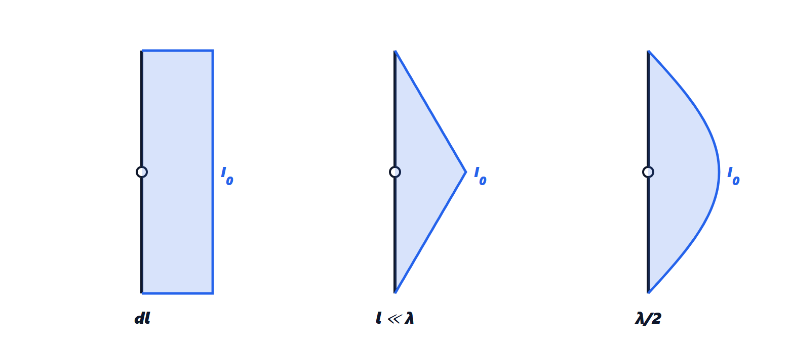
The elementary dipole

A segment with uniform current radiates in the far field

(derived in the radiation lesson from the vector potential). The power is

With (write and set ): 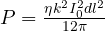. Hence

The short dipole

A real short dipole (of length ) does not have uniform current: at the ends of the wire the current must vanish, and on a short wire it decreases almost linearly, 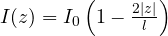. Since all segments are close compared with , the phases of the contributions are equal and the field is that of an elementary dipole with moment : the effective length is half the physical one. Substituting :

four times less than the elementary dipole of the same length. A dipole has about 2 Ω.

The half-wave dipole: the 73 Ω proved

With current for , adding the elementary dipoles with their phases gives (dipoles lesson)

The power is

and the integral, often said to be “numerical only”, can be computed exactly.

Theorem. , where 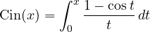is the cosine integral.

Proof. Set , , and multiply and divide by : the integral becomes 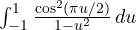. With and the partial fractions :

because the change turns the first term into the second. Now : , , and the limits become 0 and . The result is . ∎

(the function is tabulated, and near the integrand tends to zero, so there are no convergence problems). Hence

Note that the short-dipole approximation, Ω, would be 33 % wrong here: at half a wavelength the phases of the contributions are no longer equal.

Directivity. The maximum radiation intensity (at °) is , so

i.e. 2.15 dBi, the value used to define dBd. The same calculation for the elementary dipole, with 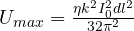, gives .

The monopole. A monopole over a conducting plane produces, above the plane, the same field as the half-wave dipole (image theorem), but radiates only into the upper half-space: half the power with the same current, hence Ω.

The dipole of any length

For a thin dipole of length with current , the same procedure gives the resistance referred to the current maximum:

The resistance seen at the terminals is , because for the same power the current at the centre is . For the current at the centre vanishes and becomes theoretically infinite: the centre-fed full-wave dipole is high impedance (in practice a few thousand ohms, because the wire has thickness).

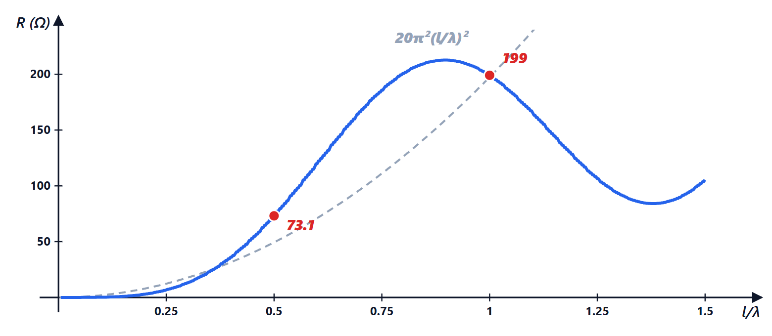
	0.1	0.25	0.5	1	1.5
(Ω)	0.19	6.72	73.1	199	105
(Ω)	2.00	13.4	73.1		105
(Ω)	1.97	12.3	49.3

The short-dipole formula (referred to the terminal current) is good up to and is already 8 % wrong at .

Losses and efficiency

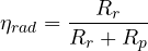
The wire has an ohmic resistance , and the supplied power splits between radiation and heat:

Skin-effect losses. At radio frequencies the current flows in a surface layer; a wire of radius and length has resistance , with the surface resistance. With sinusoidal current the dissipated power, referred to , is half that with uniform current (the average value of is 1/2). For a copper half-wave dipole ( S/m) at 100 MHz, with mm: mΩ, Ω, efficiency 99.6 %.

The short antenna. A whip of m over a ground plane at 1 MHz (medium wave, m) is a short monopole: half of a short dipole of length , i.e. mΩ. With just 1 Ω of losses (loading coil, contacts, ground) the efficiency is 0.44 %. This is why medium-wave broadcast antennas are masts tens of metres tall, and why an AM radio in a car works only because the receiver has a lot of gain and external noise dominates anyway.

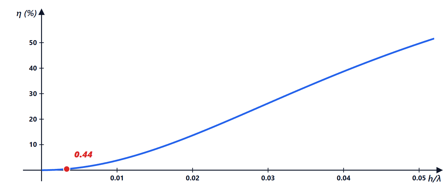
The calculation in Python

import numpy as np
from scipy.integrate import quad

eta = 120 * np.pi                                    # impedance of free space (approximate) [ohm]

# cosine integral Cin(x) = integral from 0 to x of (1 - cos t)/t
Cin = lambda x: quad(lambda t: (1 - np.cos(t)) / t, 0, x)[0]
print(f"Cin(2 pi) = {Cin(2 * np.pi):.4f} -> R = 30 Cin(2 pi) = {30 * Cin(2 * np.pi):.2f} ohm")

def R_max(l_over_lambda):
    """Radiation resistance of a thin dipole of length l, referred to the current maximum."""
    kl2 = np.pi * l_over_lambda                      # k l / 2
    f = lambda th: (np.cos(kl2 * np.cos(th)) - np.cos(kl2)) ** 2 / np.sin(th)
    return eta / (2 * np.pi) * quad(f, 1e-9, np.pi - 1e-9, limit=200)[0]

for x in (0.01, 0.1, 0.25, 0.5, 1.0, 1.5):
    Rm = R_max(x)
    s2 = np.sin(np.pi * x) ** 2
    Rin = Rm / s2 if s2 > 1e-6 else float("inf")
    print(f"l = {x:4.2f} lambda: R (I max) = {Rm:8.3f} ohm, R input = {Rin:9.3f} ohm, short 20 pi^2 x^2 = {20 * np.pi**2 * x**2:.4f}")

# directivity of the half-wave dipole: D = 4 pi U_max / P = eta / (pi R)
R05 = R_max(0.5)
print(f"D (half-wave) = {eta / (np.pi * R05):.3f} = {10 * np.log10(eta / (np.pi * R05)):.2f} dBi; lambda/4 monopole: {R05 / 2:.2f} ohm")

# 1 m whip at 1 MHz (short monopole) and 1 ohm of loss resistance
h, lam = 1.0, 300.0
Rr = 40 * np.pi**2 * (h / lam) ** 2
print(f"1 m whip at 1 MHz: Rr = {Rr * 1e3:.2f} mohm, efficiency with 1 ohm of losses = {100 * Rr / (Rr + 1):.2f} %")

# ohmic losses of a copper half-wave dipole at 100 MHz, radius 1 mm (skin effect)
f0, a, sigma, mu0 = 100e6, 1e-3, 5.8e7, 4e-7 * np.pi
Rs = np.sqrt(np.pi * f0 * mu0 / sigma)               # surface resistance [ohm]
l = 3e8 / f0 / 2
R_unif = l * Rs / (2 * np.pi * a)                    # if the current were uniform
R_loss = R_unif / 2                                  # sinusoidal current: average of cos^2 = 1/2
print(f"Rs = {Rs * 1e3:.2f} mohm, loss R = {R_loss * 1e3:.1f} mohm, efficiency = {100 * R05 / (R05 + R_loss):.2f} %")

Running it prints and Ω, the table of the previous section, (2.15 dBi), 36.56 Ω for the monopole, 4.39 mΩ and 0.44 % for the whip, 311 mΩ and 99.58 % for the copper dipole. In MATLAB the same calculation is done with integral, and the Antenna Toolbox computes the complete impedance (including the reactance, not covered here) with the method of moments.